Wrangling data with dplyr

2025-08-09

Art by Allison Horst

The main verbs of dplyr

select()

filter()

mutate()

arrange()

summarize()

group_by()

The main verbs of dplyr

select() = Subset columns (variables)

filter()

mutate()

arrange()

summarize()

group_by()

select()

select(<DATA>, <VARIABLES>)

select()

diamonds

# A tibble: 53,940 × 10
   carat cut     color clarity depth table price     x     y
   <dbl> <ord>   <ord> <ord>   <dbl> <dbl> <int> <dbl> <dbl>
 1  0.23 Ideal   E     SI2      61.5    55   326  3.95  3.98
 2  0.21 Premium E     SI1      59.8    61   326  3.89  3.84
 3  0.23 Good    E     VS1      56.9    65   327  4.05  4.07
 4  0.29 Premium I     VS2      62.4    58   334  4.2   4.23
 5  0.31 Good    J     SI2      63.3    58   335  4.34  4.35
 6  0.24 Very G… J     VVS2     62.8    57   336  3.94  3.96
 7  0.24 Very G… I     VVS1     62.3    57   336  3.95  3.98
 8  0.26 Very G… H     SI1      61.9    55   337  4.07  4.11
 9  0.22 Fair    E     VS2      65.1    61   337  3.87  3.78
10  0.23 Very G… H     VS1      59.4    61   338  4     4.05
# ℹ 53,930 more rows
# ℹ 1 more variable: z <dbl>

select()

select(diamonds, carat, cut, color, clarity)

select()

select(diamonds, carat, cut, color, clarity)

# A tibble: 53,940 × 4
   carat cut       color clarity
   <dbl> <ord>     <ord> <ord>  
 1  0.23 Ideal     E     SI2    
 2  0.21 Premium   E     SI1    
 3  0.23 Good      E     VS1    
 4  0.29 Premium   I     VS2    
 5  0.31 Good      J     SI2    
 6  0.24 Very Good J     VVS2   
 7  0.24 Very Good I     VVS1   
 8  0.26 Very Good H     SI1    
 9  0.22 Fair      E     VS2    
10  0.23 Very Good H     VS1    
# ℹ 53,930 more rows

select()

select(diamonds, carat, cut, color, clarity)
select(diamonds, carat:clarity)
select(diamonds, 1:4)
select(diamonds, starts_with("c"))
?select_helpers

gapminder

library(gapminder)
gapminder

# A tibble: 1,704 × 6
   country     continent  year lifeExp      pop gdpPercap
   <fct>       <fct>     <int>   <dbl>    <int>     <dbl>
 1 Afghanistan Asia       1952    28.8  8425333      779.
 2 Afghanistan Asia       1957    30.3  9240934      821.
 3 Afghanistan Asia       1962    32.0 10267083      853.
 4 Afghanistan Asia       1967    34.0 11537966      836.
 5 Afghanistan Asia       1972    36.1 13079460      740.
 6 Afghanistan Asia       1977    38.4 14880372      786.
 7 Afghanistan Asia       1982    39.9 12881816      978.
 8 Afghanistan Asia       1987    40.8 13867957      852.
 9 Afghanistan Asia       1992    41.7 16317921      649.
10 Afghanistan Asia       1997    41.8 22227415      635.
# ℹ 1,694 more rows

Your Turn 1

Alter the code to select just the pop column:

select(gapminder, year, lifeExp)

Your Turn 1

select(gapminder, pop)

# A tibble: 1,704 × 1
        pop
      <int>
 1  8425333
 2  9240934
 3 10267083
 4 11537966
 5 13079460
 6 14880372
 7 12881816
 8 13867957
 9 16317921
10 22227415
# ℹ 1,694 more rows

Make a prediction

Which of these is NOT a way to select the country and continent columns together?

select(gapminder, -c(year, lifeExp, pop, gdpPercap))

select(gapminder, country:continent)

select(gapminder, starts_with("c"))

select(gapminder, ends_with("t"))

Make a prediction

Which of these is NOT a way to select the country and continent columns together?

select(gapminder, ends_with("t"))

# A tibble: 1,704 × 1
   continent
   <fct>    
 1 Asia     
 2 Asia     
 3 Asia     
 4 Asia     
 5 Asia     
 6 Asia     
 7 Asia     
 8 Asia     
 9 Asia     
10 Asia     
# ℹ 1,694 more rows

The main verbs of dplyr

select()

filter() = Subset rows by value

mutate()

arrange()

summarize()

group_by()

filter()

filter(<DATA>, <PREDICATES>)

Predicates: TRUE or FALSE statements

Comparisons: >, >=, <, <=, != (not equal), and == (equal).

Operators: & is “and”, | is “or”, and ! is “not”

%in%

"a" %in% c("a", "b", "c")

[1] TRUE

filter()

filter(diamonds, cut == "Ideal", carat > 3)

# A tibble: 4 × 10
  carat cut   color clarity depth table price     x     y
  <dbl> <ord> <ord> <ord>   <dbl> <dbl> <int> <dbl> <dbl>
1  3.22 Ideal I     I1       62.6    55 12545  9.49  9.42
2  3.5  Ideal H     I1       62.8    57 12587  9.65  9.59
3  3.01 Ideal J     SI2      61.7    58 16037  9.25  9.2 
4  3.01 Ideal J     I1       65.4    60 16538  8.99  8.93
# ℹ 1 more variable: z <dbl>

Your turn 2

Show:

All of the rows where pop is greater than or equal to 100000

All of the rows for El Salvador

All of the rows that have a missing value for year (no need to edit this code)

Your turn 2

Show:

All of the rows where pop is greater than or equal to 100000

All of the rows for El Salvador

All of the rows that have a missing value for year (no need to edit this code)

filter(gapminder, pop >= 100000)
filter(gapminder, country == "El Salvador")
filter(gapminder, is.na(year))

filter()

filter(diamonds, cut == "Ideal" | cut == "Very Good", carat > 3)

# A tibble: 6 × 10
  carat cut      color clarity depth table price     x     y
  <dbl> <ord>    <ord> <ord>   <dbl> <dbl> <int> <dbl> <dbl>
1  3.22 Ideal    I     I1       62.6    55 12545  9.49  9.42
2  3.5  Ideal    H     I1       62.8    57 12587  9.65  9.59
3  3.04 Very Go… I     SI2      63.2    59 15354  9.14  9.07
4  4    Very Go… I     I1       63.3    58 15984 10.0   9.94
5  3.01 Ideal    J     SI2      61.7    58 16037  9.25  9.2 
6  3.01 Ideal    J     I1       65.4    60 16538  8.99  8.93
# ℹ 1 more variable: z <dbl>

Your turn 3

Use Boolean operators to alter the code below to return only the rows that contain:

El Salvador

Countries that had populations over 100000 in 1960 or earlier

filter(gapminder, country == "El Salvador" | country == "Oman")
filter(______, _______)

Your turn 3

Use Boolean operators to alter the code below to return only the rows that contain:

El Salvador

Countries that had populations over 100000 in 1960 or earlier

filter(gapminder, country == "El Salvador")
filter(gapminder, pop > 100000, year <= 1960)

The main verbs of dplyr

select()

filter()

mutate() = Change or add a variable

arrange()

summarize()

group_by()

mutate()

mutate(<DATA>, <NAME> = <FUNCTION>)

mutate()

mutate(
  diamonds, 
  log_price = log(price), 
  log_pricesq = log_price^2
)

mutate()

# A tibble: 53,940 × 12
   carat cut     color clarity depth table price     x     y
   <dbl> <ord>   <ord> <ord>   <dbl> <dbl> <int> <dbl> <dbl>
 1  0.23 Ideal   E     SI2      61.5    55   326  3.95  3.98
 2  0.21 Premium E     SI1      59.8    61   326  3.89  3.84
 3  0.23 Good    E     VS1      56.9    65   327  4.05  4.07
 4  0.29 Premium I     VS2      62.4    58   334  4.2   4.23
 5  0.31 Good    J     SI2      63.3    58   335  4.34  4.35
 6  0.24 Very G… J     VVS2     62.8    57   336  3.94  3.96
 7  0.24 Very G… I     VVS1     62.3    57   336  3.95  3.98
 8  0.26 Very G… H     SI1      61.9    55   337  4.07  4.11
 9  0.22 Fair    E     VS2      65.1    61   337  3.87  3.78
10  0.23 Very G… H     VS1      59.4    61   338  4     4.05
# ℹ 53,930 more rows
# ℹ 3 more variables: z <dbl>, log_price <dbl>,
#   log_pricesq <dbl>

The main verbs of dplyr

select()

filter()

mutate()

arrange() = Sort the data set

summarize()

group_by()

arrange()

arrange(<DATA>, <SORTING VARIABLE>)

arrange()

arrange(diamonds, price)

# A tibble: 53,940 × 10
   carat cut     color clarity depth table price     x     y
   <dbl> <ord>   <ord> <ord>   <dbl> <dbl> <int> <dbl> <dbl>
 1  0.23 Ideal   E     SI2      61.5    55   326  3.95  3.98
 2  0.21 Premium E     SI1      59.8    61   326  3.89  3.84
 3  0.23 Good    E     VS1      56.9    65   327  4.05  4.07
 4  0.29 Premium I     VS2      62.4    58   334  4.2   4.23
 5  0.31 Good    J     SI2      63.3    58   335  4.34  4.35
 6  0.24 Very G… J     VVS2     62.8    57   336  3.94  3.96
 7  0.24 Very G… I     VVS1     62.3    57   336  3.95  3.98
 8  0.26 Very G… H     SI1      61.9    55   337  4.07  4.11
 9  0.22 Fair    E     VS2      65.1    61   337  3.87  3.78
10  0.23 Very G… H     VS1      59.4    61   338  4     4.05
# ℹ 53,930 more rows
# ℹ 1 more variable: z <dbl>

arrange()

arrange(diamonds, cut, price)

# A tibble: 53,940 × 10
   carat cut   color clarity depth table price     x     y
   <dbl> <ord> <ord> <ord>   <dbl> <dbl> <int> <dbl> <dbl>
 1  0.22 Fair  E     VS2      65.1    61   337  3.87  3.78
 2  0.25 Fair  E     VS1      55.2    64   361  4.21  4.23
 3  0.23 Fair  G     VVS2     61.4    66   369  3.87  3.91
 4  0.27 Fair  E     VS1      66.4    58   371  3.99  4.02
 5  0.3  Fair  J     VS2      64.8    58   416  4.24  4.16
 6  0.3  Fair  F     SI1      63.1    58   496  4.3   4.22
 7  0.34 Fair  J     SI1      64.5    57   497  4.38  4.36
 8  0.37 Fair  F     SI1      65.3    56   527  4.53  4.47
 9  0.3  Fair  D     SI2      64.6    54   536  4.29  4.25
10  0.25 Fair  D     VS1      61.2    55   563  4.09  4.11
# ℹ 53,930 more rows
# ℹ 1 more variable: z <dbl>

desc()

arrange(diamonds, cut, desc(price))

# A tibble: 53,940 × 10
   carat cut   color clarity depth table price     x     y
   <dbl> <ord> <ord> <ord>   <dbl> <dbl> <int> <dbl> <dbl>
 1  2.01 Fair  G     SI1      70.6    64 18574  7.43  6.64
 2  2.02 Fair  H     VS2      64.5    57 18565  8     7.95
 3  4.5  Fair  J     I1       65.8    58 18531 10.2  10.2 
 4  2    Fair  G     VS2      67.6    58 18515  7.65  7.61
 5  2.51 Fair  H     SI2      64.7    57 18308  8.44  8.5 
 6  3.01 Fair  I     SI2      65.8    56 18242  8.99  8.94
 7  3.01 Fair  I     SI2      65.8    56 18242  8.99  8.94
 8  2.32 Fair  H     SI1      62      62 18026  8.47  8.31
 9  5.01 Fair  J     I1       65.5    59 18018 10.7  10.5 
10  1.93 Fair  F     VS1      58.9    62 17995  8.17  7.97
# ℹ 53,930 more rows
# ℹ 1 more variable: z <dbl>

Your turn 4

Arrange gapminder by year. Add lifeExp as a second (tie breaking) variable to arrange on.

Which country had the lowest life expectancy in 1952?

Your turn 4

arrange(gapminder, year, lifeExp)

# A tibble: 1,704 × 6
   country       continent  year lifeExp     pop gdpPercap
   <fct>         <fct>     <int>   <dbl>   <int>     <dbl>
 1 Afghanistan   Asia       1952    28.8 8425333      779.
 2 Gambia        Africa     1952    30    284320      485.
 3 Angola        Africa     1952    30.0 4232095     3521.
 4 Sierra Leone  Africa     1952    30.3 2143249      880.
 5 Mozambique    Africa     1952    31.3 6446316      469.
 6 Burkina Faso  Africa     1952    32.0 4469979      543.
 7 Guinea-Bissau Africa     1952    32.5  580653      300.
 8 Yemen, Rep.   Asia       1952    32.5 4963829      782.
 9 Somalia       Africa     1952    33.0 2526994     1136.
10 Guinea        Africa     1952    33.6 2664249      510.
# ℹ 1,694 more rows

Your turn 5

Use desc() to find the country with the highest gdpPercap.

Your turn 5

arrange(gapminder, desc(gdpPercap))

# A tibble: 1,704 × 6
   country   continent  year lifeExp     pop gdpPercap
   <fct>     <fct>     <int>   <dbl>   <int>     <dbl>
 1 Kuwait    Asia       1957    58.0  212846   113523.
 2 Kuwait    Asia       1972    67.7  841934   109348.
 3 Kuwait    Asia       1952    55.6  160000   108382.
 4 Kuwait    Asia       1962    60.5  358266    95458.
 5 Kuwait    Asia       1967    64.6  575003    80895.
 6 Kuwait    Asia       1977    69.3 1140357    59265.
 7 Norway    Europe     2007    80.2 4627926    49357.
 8 Kuwait    Asia       2007    77.6 2505559    47307.
 9 Singapore Asia       2007    80.0 4553009    47143.
10 Norway    Europe     2002    79.0 4535591    44684.
# ℹ 1,694 more rows

Detour: The Pipe |>

Detour: The Pipe

diamonds <- arrange(diamonds, price)
diamonds <- filter(diamonds, price > 300)
diamonds <- mutate(diamonds, log_price = log(price))

diamonds

Detour: The Pipe

diamonds <- diamonds |> 
  arrange(price) |> 
  filter(price > 300) |> 
  mutate(log_price = log(price))

diamonds

Passes the result of one function to another function

Keyboard shortcuts

Insert <- with alt/opt + -

Insert |> with ctrl/cmd + shift + m

Keyboard shortcuts

Tools > Global Options > Code

The magrittr pipe

In the wild, you’ll see %>% a lot. This is the old pipe prior to when R had a built-in one. Either pipe is fine, but we’ll use the so-called native pipe |>

See R for Data Science for more info

Your turn 6

Use |> to write a sequence of functions that:

Filter only countries that are in the continent of Oceania.

Select the country, year and lifeExp columns

Arrange the results so that the highest life expectancy is at the top.

Your turn 6

gapminder |> 
  filter(continent == "Oceania") |> 
  select(country, year, lifeExp) |> 
  arrange(desc(lifeExp))

# A tibble: 24 × 3
   country      year lifeExp
   <fct>       <int>   <dbl>
 1 Australia    2007    81.2
 2 Australia    2002    80.4
 3 New Zealand  2007    80.2
 4 New Zealand  2002    79.1
 5 Australia    1997    78.8
 6 Australia    1992    77.6
 7 New Zealand  1997    77.6
 8 New Zealand  1992    76.3
 9 Australia    1987    76.3
10 Australia    1982    74.7
# ℹ 14 more rows

Challenge!

1. Import the diabetes data from the importing data. A copy of the CSV file is available in this folder.

2. Add the variable bmi to the data set using height and weight using the formula: (weight / height^2) * 703

3. Select just id, glyhb, and the new variable you created.

4. Filter rows that have BMI > 35. How many rows and columns are in your new data set?

diabetes <- read_csv("diabetes.csv")
diabetes |> 
  mutate(bmi = (weight / height^2) * 703) |> 
  select(id, glyhb, bmi) |> 
  filter(bmi > 35)

# A tibble: 61 × 3
      id glyhb   bmi
   <dbl> <dbl> <dbl>
 1  1001  4.44  37.4
 2  1002  4.64  48.4
 3  1022  5.78  35.8
 4  1029  4.97  40.8
 5  1253  4.67  36.0
 6  1254 12.7   42.5
 7  1280  5.10  38.3
 8  1501  4.41  40.0
 9  2753  5.57  35.3
10  2757  6.33  35.3
# ℹ 51 more rows

The main verbs of dplyr

select()

filter()

mutate()

arrange()

summarize() = Summarize the data

group_by() = Group the data

summarize()

summarize(<DATA>, <NAME> = <FUNCTION>)

summarize()

summarize(diamonds, n = n(), mean_price = mean(price))

# A tibble: 1 × 2
      n mean_price
  <int>      <dbl>
1 53940      3933.

Your turn 7

Use summarise() to compute these statistics about the gapminder data set:

1. The first (min()) year in the data

2. The last (max()) year in the data

3. The total number of observations (n()) and the total number of unique countries in the data (n_distinct())

Your turn 7

gapminder |> 
  summarize(
    first = min(year), 
    last = max(year), 
    n = n(), 
    n_countries = n_distinct(country)
  )

# A tibble: 1 × 4
  first  last     n n_countries
  <int> <int> <int>       <int>
1  1952  2007  1704         142

group_by()

group_by(<DATA>, <VARIABLE>)

group_by()

diamonds |> 
  group_by(cut)

# A tibble: 53,940 × 10
# Groups:   cut [5]
   carat cut     color clarity depth table price     x     y
   <dbl> <ord>   <ord> <ord>   <dbl> <dbl> <int> <dbl> <dbl>
 1  0.23 Ideal   E     SI2      61.5    55   326  3.95  3.98
 2  0.21 Premium E     SI1      59.8    61   326  3.89  3.84
 3  0.23 Good    E     VS1      56.9    65   327  4.05  4.07
 4  0.29 Premium I     VS2      62.4    58   334  4.2   4.23
 5  0.31 Good    J     SI2      63.3    58   335  4.34  4.35
 6  0.24 Very G… J     VVS2     62.8    57   336  3.94  3.96
 7  0.24 Very G… I     VVS1     62.3    57   336  3.95  3.98
 8  0.26 Very G… H     SI1      61.9    55   337  4.07  4.11
 9  0.22 Fair    E     VS2      65.1    61   337  3.87  3.78
10  0.23 Very G… H     VS1      59.4    61   338  4     4.05
# ℹ 53,930 more rows
# ℹ 1 more variable: z <dbl>

group_by()

diamonds |> 
  group_by(cut) |> 
  summarize(n = n(), mean_price = mean(price)) 

# A tibble: 5 × 3
  cut           n mean_price
  <ord>     <int>      <dbl>
1 Fair       1610      4359.
2 Good       4906      3929.
3 Very Good 12082      3982.
4 Premium   13791      4584.
5 Ideal     21551      3458.

Your turn 8

Extract the rows where continent == "Europe". Then use group_by() to group by country. Finally, use summarize() to compute:

1. The total number of observations for each country in Europe

2. The lowest observed life expectancy for each country

Your turn 8

gapminder |> 
  filter(continent == "Europe") |> 
  group_by(country) |> 
  summarize(n = n(), min_le = min(lifeExp))

# A tibble: 30 × 3
   country                    n min_le
   <fct>                  <int>  <dbl>
 1 Albania                   12   55.2
 2 Austria                   12   66.8
 3 Belgium                   12   68  
 4 Bosnia and Herzegovina    12   53.8
 5 Bulgaria                  12   59.6
 6 Croatia                   12   61.2
 7 Czech Republic            12   66.9
 8 Denmark                   12   70.8
 9 Finland                   12   66.6
10 France                    12   67.4
# ℹ 20 more rows

Your turn 9

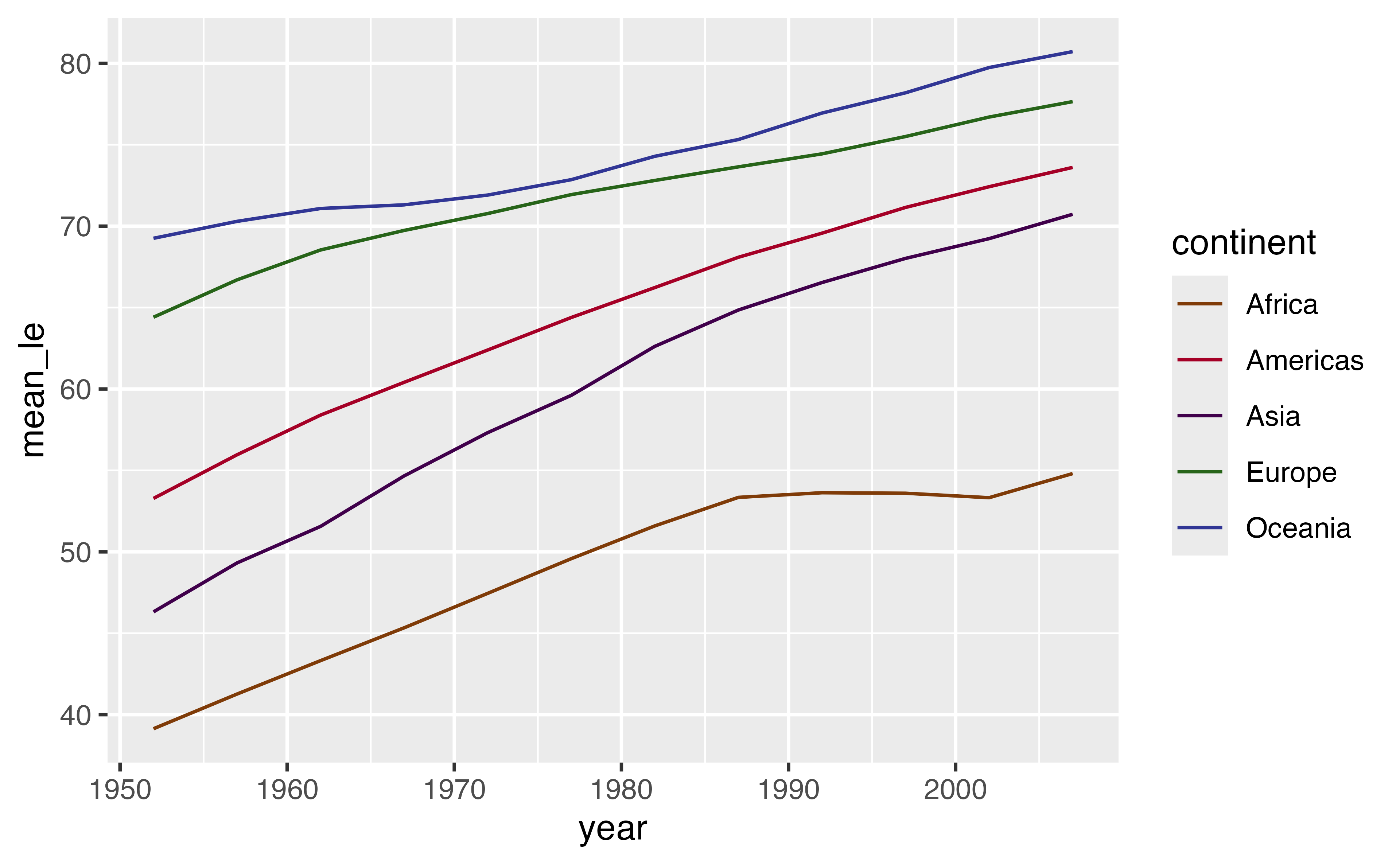
Use grouping to calculate the mean life expectancy for each continent and year. Call the mean life expectancy variable mean_le. Plot the life expectancy over time (no need to change the plot code).

gapminder |> 
  __________ |> 
  __________ |> 
  ggplot(aes(x = year, y = mean_le, col = continent)) +
  geom_line() + 
  scale_color_manual(values = continent_colors)

Your turn 9

Use grouping to calculate the mean life expectancy for each continent and year. Call the mean life expectancy variable mean_le. Plot the life expectancy over time (no need to change the plot code).

gapminder |> 
  group_by(continent, year) |> 
  summarize(mean_le = mean(lifeExp)) |> 
  ggplot(aes(x = year, y = mean_le, col = continent)) +
  geom_line() + 
  scale_color_manual(values = continent_colors)

Joining data

Use left_join(), right_join(), full_join(), or inner_join() to join datasets

Use semi_join() or anti_join() to filter datasets against each other

Resources

R for Data Science: A comprehensive but friendly introduction to the tidyverse. Free online.

Posit Recipes: Common code patterns in R (with some comparisons to SAS)