
Modeling in R and Tidying Results
linear models and broom
2025-08-09
Modeling in R
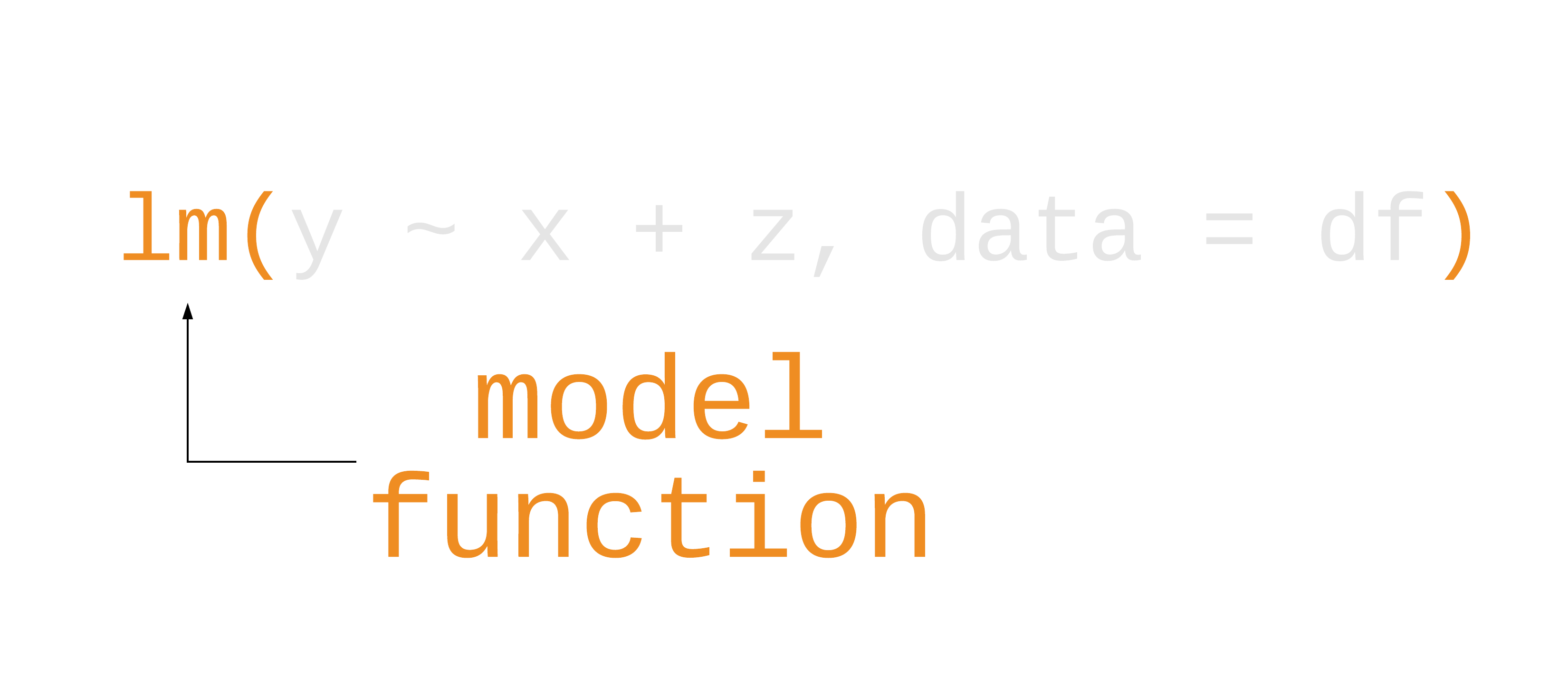
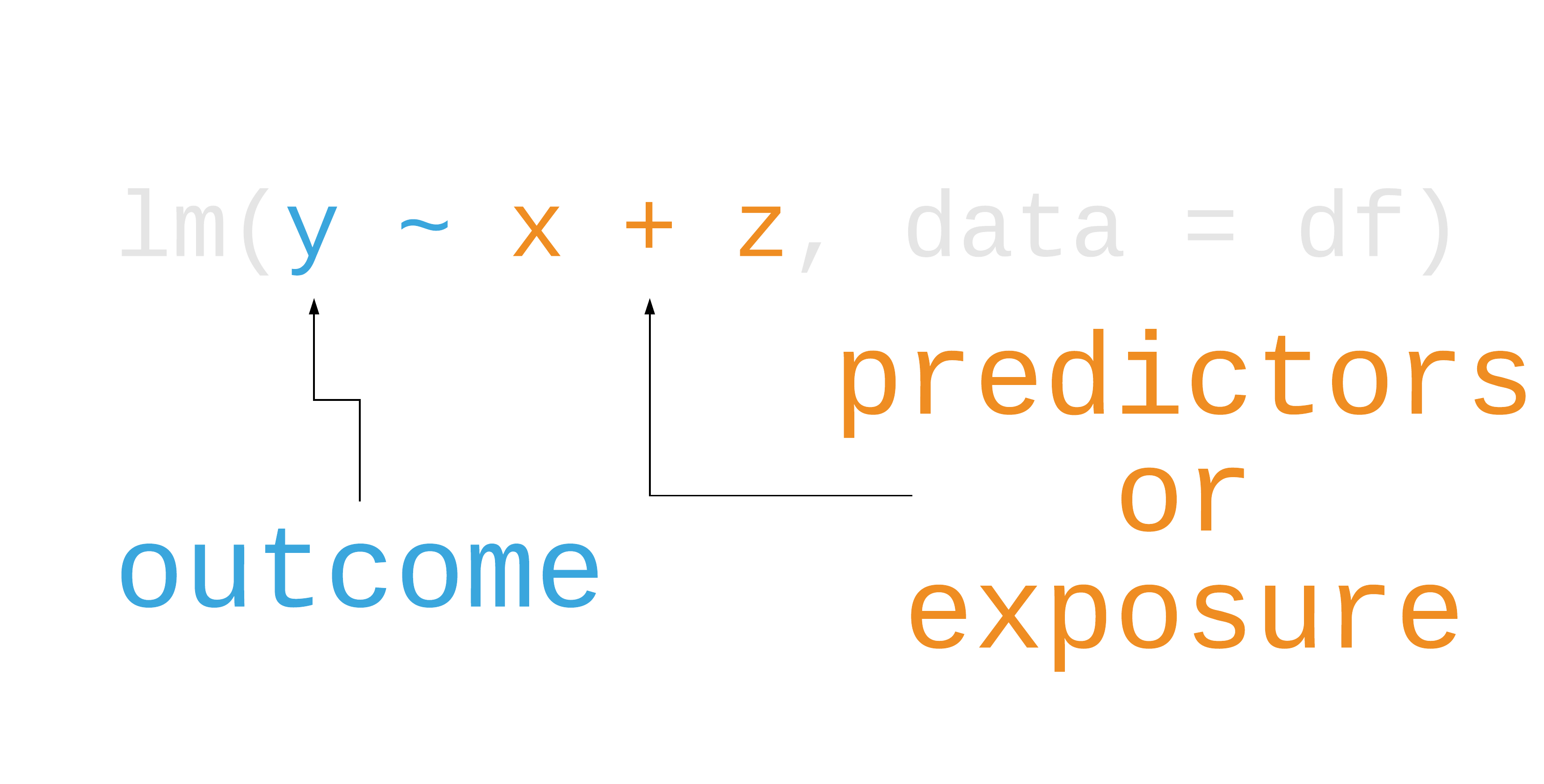
Modeling in R
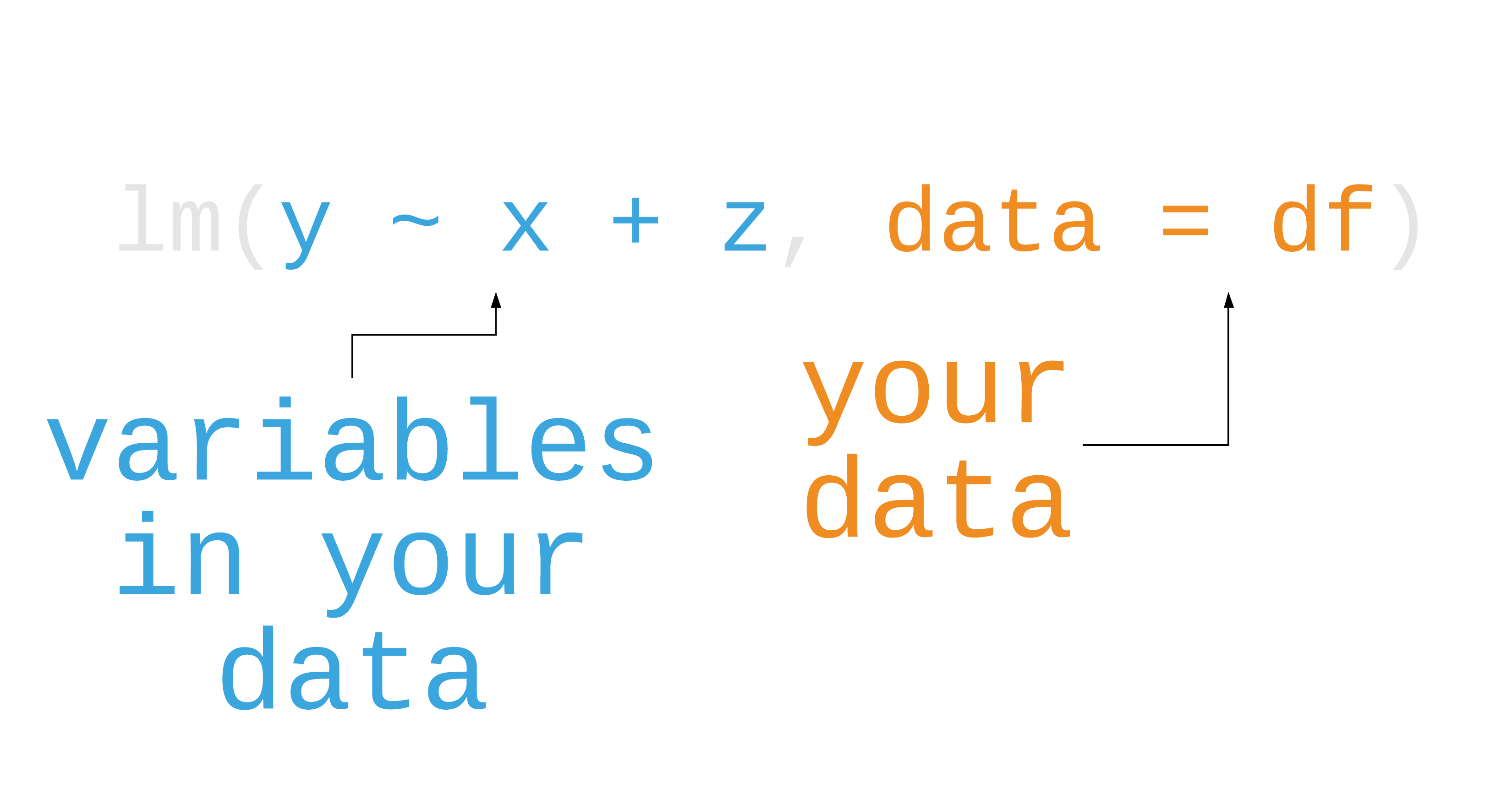
Modeling in R
broom: tidy models

tidy()
glance()
augment()
broom: tidy models
tidy() = model coefficients
glance()
glance()augment()
augment()broom: tidy models
tidy()
tidy()glance() = model fit
augment()
augment()broom: tidy models
tidy()
tidy()glance()
glance()augment() = model predictions
broom: tidy models
tidy()
tidy()glance()
glance()augment()
augment()