   char     num
"hello" "1" Functional programming in R
2025-08-09
purrr: A functional programming toolkit for R
Complete and consistent set of tools for working with functions and vectors
Problems we want to solve:
- Making code clear
- Making code safe
- Working iteratively with lists and data frames
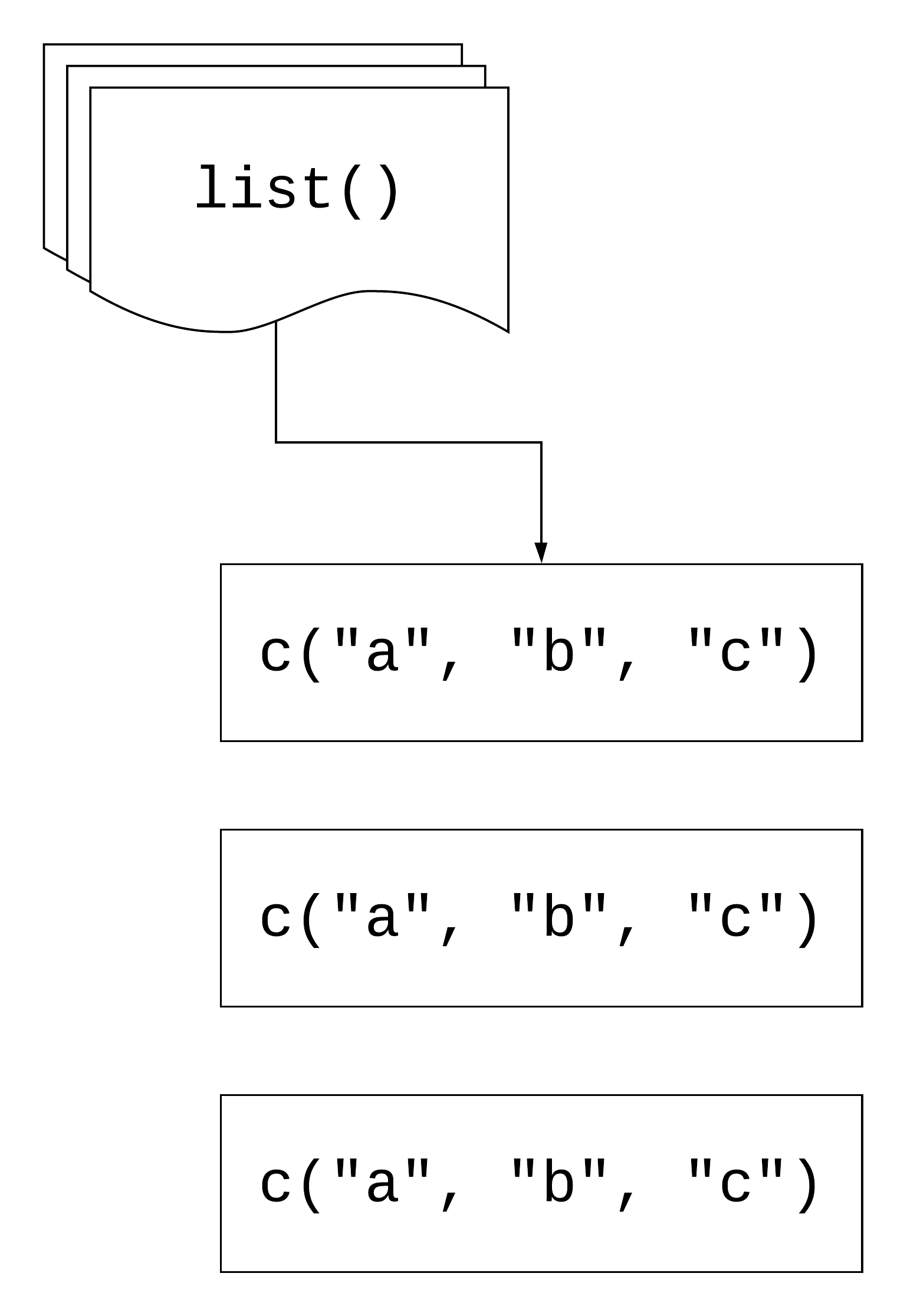
Lists, vectors, and data.frames (or tibbles)
lists can contain any object
Your Turn 1
There are two ways to subset lists: dollar signs and brackets. Try to subset blood_glucose from measurements using these approaches.
Are they different? What about measurements[["blood_glucose"]]?
Your Turn 1
$blood_glucose
 [1] 127.9293 142.7743 150.8444 116.5430 144.2912 145.0606 134.2526 134.5337
[9] 134.3555 131.0996 [1] 127.9293 142.7743 150.8444 116.5430 144.2912 145.0606 134.2526 134.5337
[9] 134.3555 131.0996 [1] 127.9293 142.7743 150.8444 116.5430 144.2912 145.0606 134.2526 134.5337
[9] 134.3555 131.0996data frames are lists
data frames are lists
data frames are lists
# A tibble: 6 × 1
       pop
     <int>
1  8425333
2  9240934
3 10267083
4 11537966
5 13079460
6 14880372
data frames are lists
programming with functions
functions are objects, too
programming with functions
source code of a function
Art by Allison Horst
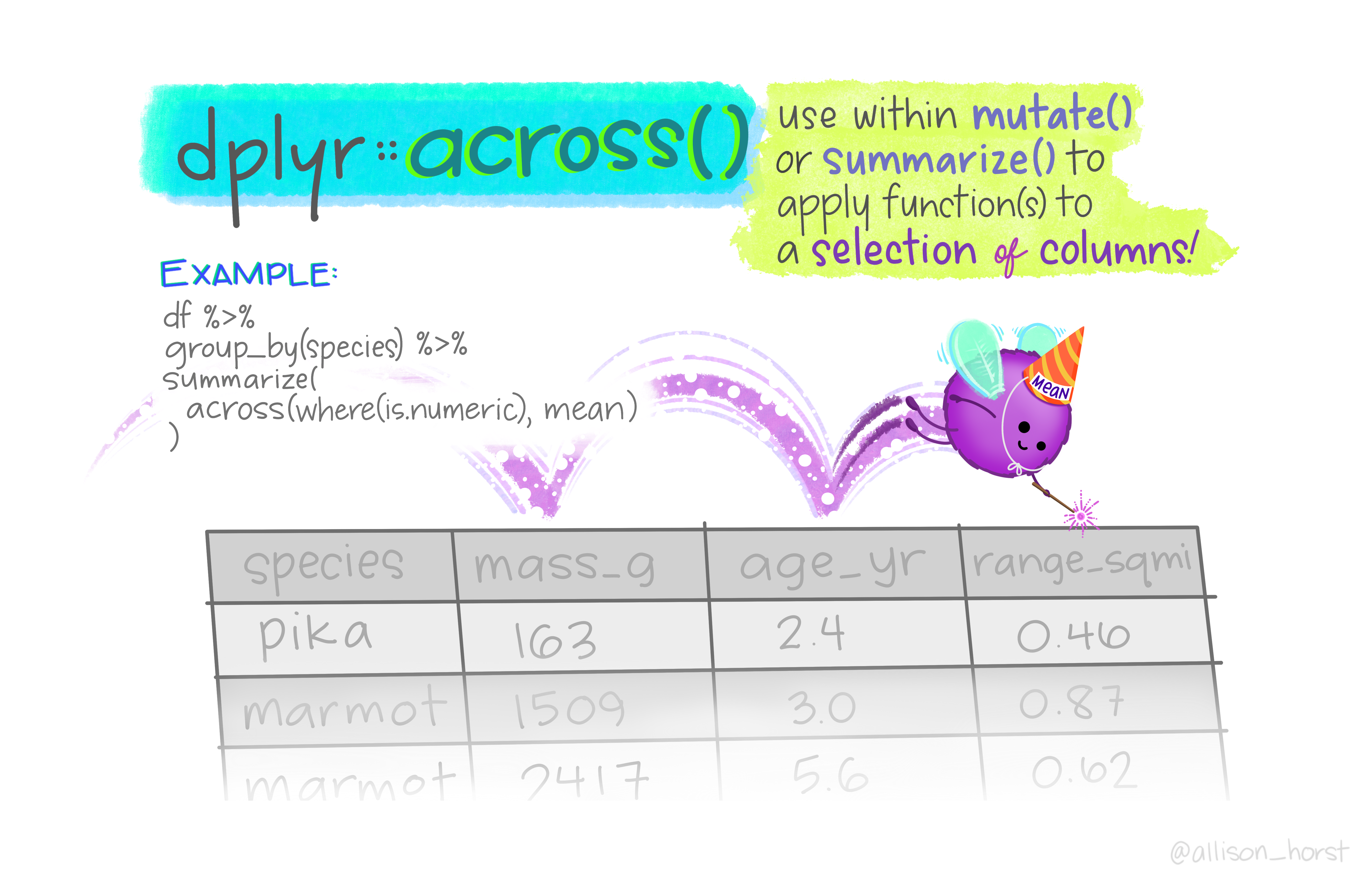
mutate(across())
mutate(across())
# A tibble: 53,940 × 10
   carat cut     color clarity depth table price     x     y
   <dbl> <ord>   <ord> <ord>   <dbl> <dbl> <int> <dbl> <dbl>
 1 0.798 Ideal   E     SI2      61.7    55   326  3.95  3.98
 2 0.798 Premium E     SI1      61.7    61   326  3.89  3.84
 3 0.798 Good    E     VS1      61.7    65   327  4.05  4.07
 4 0.798 Premium I     VS2      61.7    58   334  4.2   4.23
 5 0.798 Good    J     SI2      61.7    58   335  4.34  4.35
 6 0.798 Very G… J     VVS2     61.7    57   336  3.94  3.96
 7 0.798 Very G… I     VVS1     61.7    57   336  3.95  3.98
 8 0.798 Very G… H     SI1      61.7    55   337  4.07  4.11
 9 0.798 Fair    E     VS2      61.7    61   337  3.87  3.78
10 0.798 Very G… H     VS1      61.7    61   338  4     4.05
# ℹ 53,930 more rows
# ℹ 1 more variable: z <dbl>
mutate(across())
# A tibble: 53,940 × 14
   carat cut     color clarity depth table price     x     y
   <dbl> <ord>   <ord> <ord>   <dbl> <dbl> <int> <dbl> <dbl>
 1  0.23 Ideal   E     SI2      61.5    55   326  3.95  3.98
 2  0.21 Premium E     SI1      59.8    61   326  3.89  3.84
 3  0.23 Good    E     VS1      56.9    65   327  4.05  4.07
 4  0.29 Premium I     VS2      62.4    58   334  4.2   4.23
 5  0.31 Good    J     SI2      63.3    58   335  4.34  4.35
 6  0.24 Very G… J     VVS2     62.8    57   336  3.94  3.96
 7  0.24 Very G… I     VVS1     62.3    57   336  3.95  3.98
 8  0.26 Very G… H     SI1      61.9    55   337  4.07  4.11
 9  0.22 Fair    E     VS2      65.1    61   337  3.87  3.78
10  0.23 Very G… H     VS1      59.4    61   338  4     4.05
# ℹ 53,930 more rows
# ℹ 5 more variables: z <dbl>, carat_mean <dbl>,
#   carat_sd <dbl>, depth_mean <dbl>, depth_sd <dbl>
mutate(across(where()))
# A tibble: 1,704 × 6
   country     continent  year lifeExp      pop gdpPercap
   <fct>       <fct>     <dbl>   <dbl>    <dbl>     <dbl>
 1 Afghanistan Asia      1980.    60.7 7023596.     3532.
 2 Afghanistan Asia      1980.    60.7 7023596.     3532.
 3 Afghanistan Asia      1980.    60.7 7023596.     3532.
 4 Afghanistan Asia      1980.    60.7 7023596.     3532.
 5 Afghanistan Asia      1980.    60.7 7023596.     3532.
 6 Afghanistan Asia      1980.    60.7 7023596.     3532.
 7 Afghanistan Asia      1980.    60.7 7023596.     3532.
 8 Afghanistan Asia      1980.    60.7 7023596.     3532.
 9 Afghanistan Asia      1980.    60.7 7023596.     3532.
10 Afghanistan Asia      1980.    60.7 7023596.     3532.
# ℹ 1,694 more rows
Review: tidyselect
Workhorse for dplyr::select(), dplyr::pull(), tidyr::pivot_*(), etc.
starts_with(), ends_with(), contains(), matches(), etc.
mutate(across()) & summarise()
# A tibble: 5 × 5
  continent lifeExp_med lifeExp_iqr gdpPercap_med
  <fct>           <dbl>       <dbl>         <dbl>
1 Africa           47.8       12.0          1192.
2 Americas         67.0       13.3          5466.
3 Asia             61.8       18.1          2647.
4 Europe           72.2        5.88        12082.
5 Oceania          73.7        6.35        17983.
# ℹ 1 more variable: gdpPercap_iqr <dbl>
Your Turn 2
Use starts_with() from tidyselect() to calculate the average bp columns in diabetes, grouped by gender.
Your Turn 2
vectorized functions don’t work on lists
[1] -7.198318vectorized functions don’t work on lists
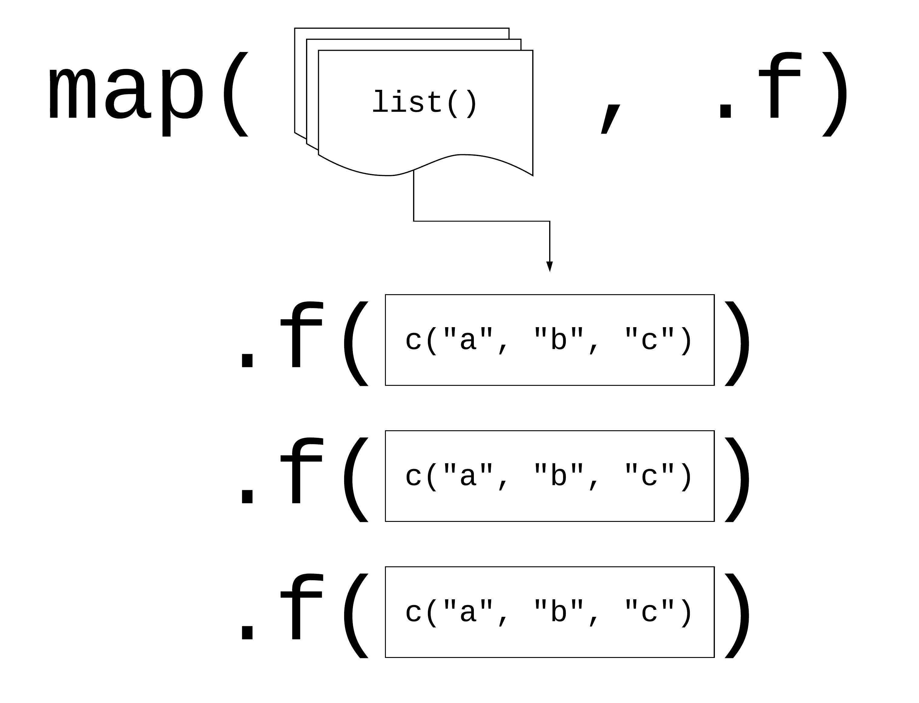
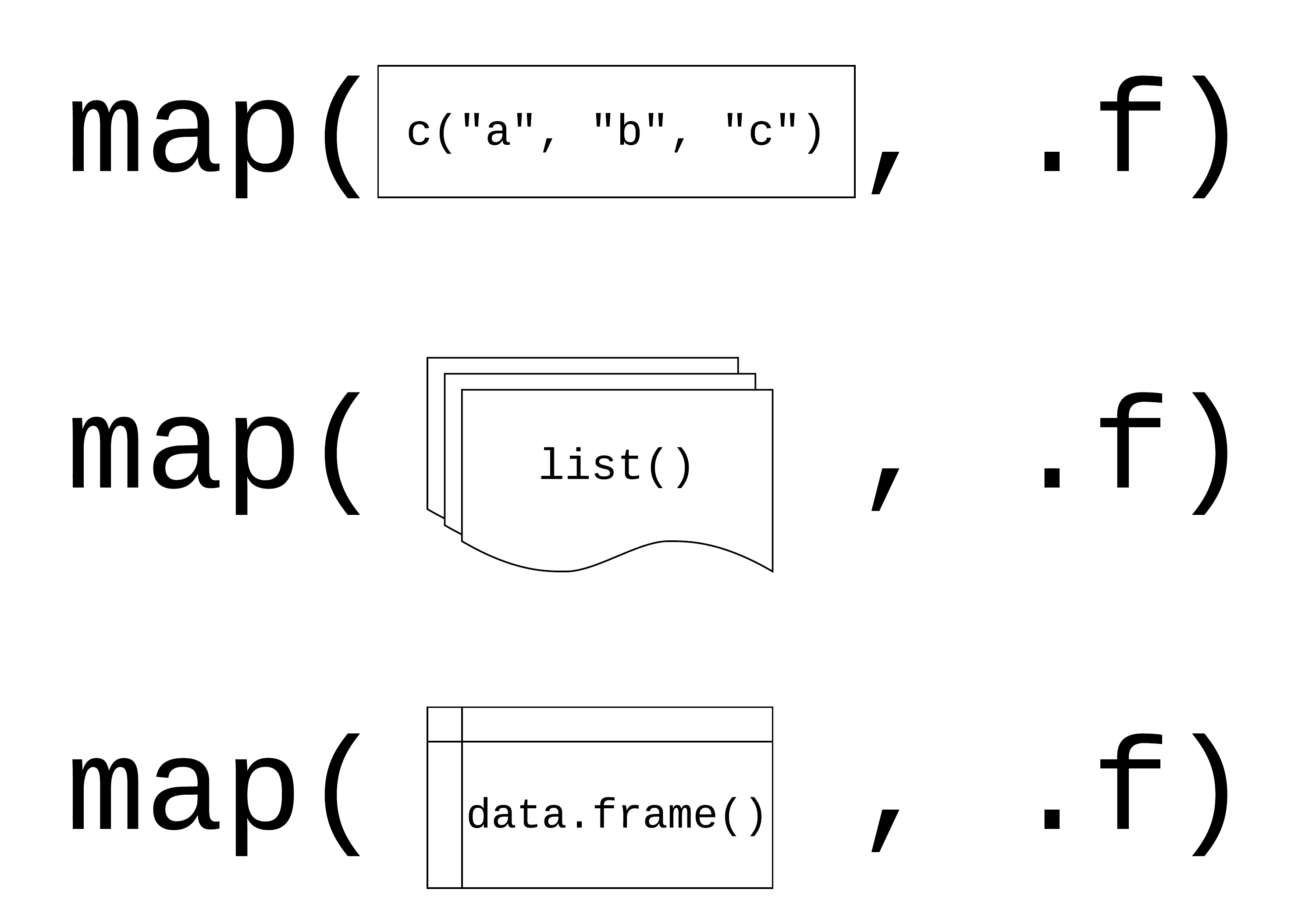
Error in sum(list(x = rnorm(10), y = rnorm(10), z = rnorm(10))): invalid 'type' (list) of argumentmap(.x, .f)
.x: a vector, list, or data frame
.f: a function
Returns a list
Using map()
Your Turn 3
Read the code in the first chunk and predict what will happen
Run the code in the first chunk. What does it return?
Now, use map() to create the same output.
Your Turn 3
using map() with data frames
$year
[1] 17.26533

$lifeExp
[1] 12.91711

$pop
[1] 106157897

$gdpPercap
[1] 9857.455
Your Turn 4
Pass diabetes to map() and map using class(). What are these results telling you?
Your Turn 4
Review: writing functions
Review: writing functionss
library(readxl)
weird_data1 <- read_excel(
  "data/weird_data1.xlsx",
  col_names = c("id", "x", "y", "z"),
  skip = 5
)
weird_data2 <- read_excel(
"data/weird_data1.xlsx",
col_names = c("id", "x", "y", "z"),
skip = 5
)
weird_data1 <- read_excel(
"data/weird_data3.xlsx",
col_names = c("id", "x", "y", "z"),
skip = 5
)Review: writing functionss
library(readxl)
weird_data1 <- read_excel(
  "data/weird_data1.xlsx",
  sheet = 2,
  col_names = c("id", "x", "y", "z"),
  skip = 6
)

weird_data2 <- read_excel(
  "data/weird_data1.xlsx",
  col_names = c("id", "x", "y", "z"),
  skip = 5
)

weird_data1 <- read_excel(
  "data/weird_data3.xlsx",
  col_names = c("id", "x", "y", "z"),
  skip = 5
)
Review: writing functions
If you copy and paste your code three times, it’s time to write a function
If you copy and paste your function three times, it’s (probably) time to iterate
Iterating with functions
Your Turn 5
Write a function that returns the mean and standard deviation of a numeric vector.
Give the function a name
Find the mean and SD of x
Map your function to measurements
Your Turn 5
Your Turn 5
$blood_glucose
# A tibble: 1 × 2
   mean    sd
  <dbl> <dbl>
1  137.  6.84

$age
# A tibble: 1 × 2
   mean    sd
  <dbl> <dbl>
1  39.5  3.84

$heartrate
# A tibble: 1 × 2
   mean    sd
  <dbl> <dbl>
1  83.0  12.6
Three ways to pass functions to map()
- pass directly to
map() - use an anonymous function
- use a lambda (
\()or~)
$country
[1] 142

$continent
[1] 5

$year
[1] 12

$lifeExp
[1] 1626

$pop
[1] 1704

$gdpPercap
[1] 1704
Returning types
| map | returns |
|---|---|
map() |
list |
map_chr() |
character vector |
map_dbl() |
double vector (numeric) |
map_int() |
integer vector |
map_lgl() |
logical vector |
map_dfc() |
data frame (by column) |
map_dfr() |
data frame (by row) |
Iterating with functions: revisited
Iterating with functions: revisited
Returning types
  country continent      year   lifeExp       pop gdpPercap
      142         5        12      1626      1704      1704
Your Turn 6
Do the same as #4 above but return a vector instead of a list.
Your Turn 6
         id        chol    stab.glu         hdl       ratio       glyhb
  "numeric"   "numeric"   "numeric"   "numeric"   "numeric"   "numeric"
   location         age      gender      height      weight       frame
"character"   "numeric" "character"   "numeric"   "numeric" "character"
      bp.1s       bp.1d       bp.2s       bp.2d       waist         hip
  "numeric"   "numeric"   "numeric"   "numeric"   "numeric"   "numeric"
   time.ppn
  "numeric"
Your Turn 7
Check diabetes for any missing data.
Using the \(.x) .f(.x) shorthand, check each column for any missing values using is.na() and any()
Return a logical vector. Are any columns missing data? What happens if you don’t include any()? Why?
Try counting the number of missing, returning an integer vector
Your Turn 7
Your Turn 7
group_map()
Apply a function across a grouping variable and return a list of grouped tibbles
group_map()
[[1]]
# A tibble: 2 × 5
  term        estimate std.error statistic   p.value
  <chr>          <dbl>     <dbl>     <dbl>     <dbl>
1 (Intercept)   -73.8     59.2       -1.25 0.214
2 height          3.90     0.928      4.20 0.0000383

[[2]]
# A tibble: 2 × 5
  term        estimate std.error statistic  p.value
  <chr>          <dbl>     <dbl>     <dbl>    <dbl>
1 (Intercept)   -49.7     68.9      -0.722 0.471
2 height          3.35     0.995     3.37  0.000945
group_modify()
Apply a function across grouped tibbles and return grouped tibbles
# A tibble: 4 × 6
# Groups:   gender [2]
  gender term        estimate std.error statistic   p.value
  <chr>  <chr>          <dbl>     <dbl>     <dbl>     <dbl>
1 female (Intercept)   -73.8     59.2      -1.25  0.214
2 female height          3.90     0.928     4.20  0.0000383
3 male   (Intercept)   -49.7     68.9      -0.722 0.471
4 male   height          3.35     0.995     3.37  0.000945
Your Turn 8
Fill in the model_lm function to model chol (the outcome) with ratio and pass the .data argument to lm()
Group diabetes by location
Use group_modify() with model_lm
Your Turn 8
Your Turn 8
# A tibble: 2 × 13
# Groups: location [2]
location r.squared adj.r.squared sigma statistic p.value
<chr> <dbl> <dbl> <dbl> <dbl> <dbl>
1 Buckingh… 0.252 0.248 38.8 66.4 4.11e-14
2 Louisa 0.204 0.201 39.4 51.7 1.26e-11
# ℹ 7 more variables: df <dbl>, logLik <dbl>, AIC <dbl>,
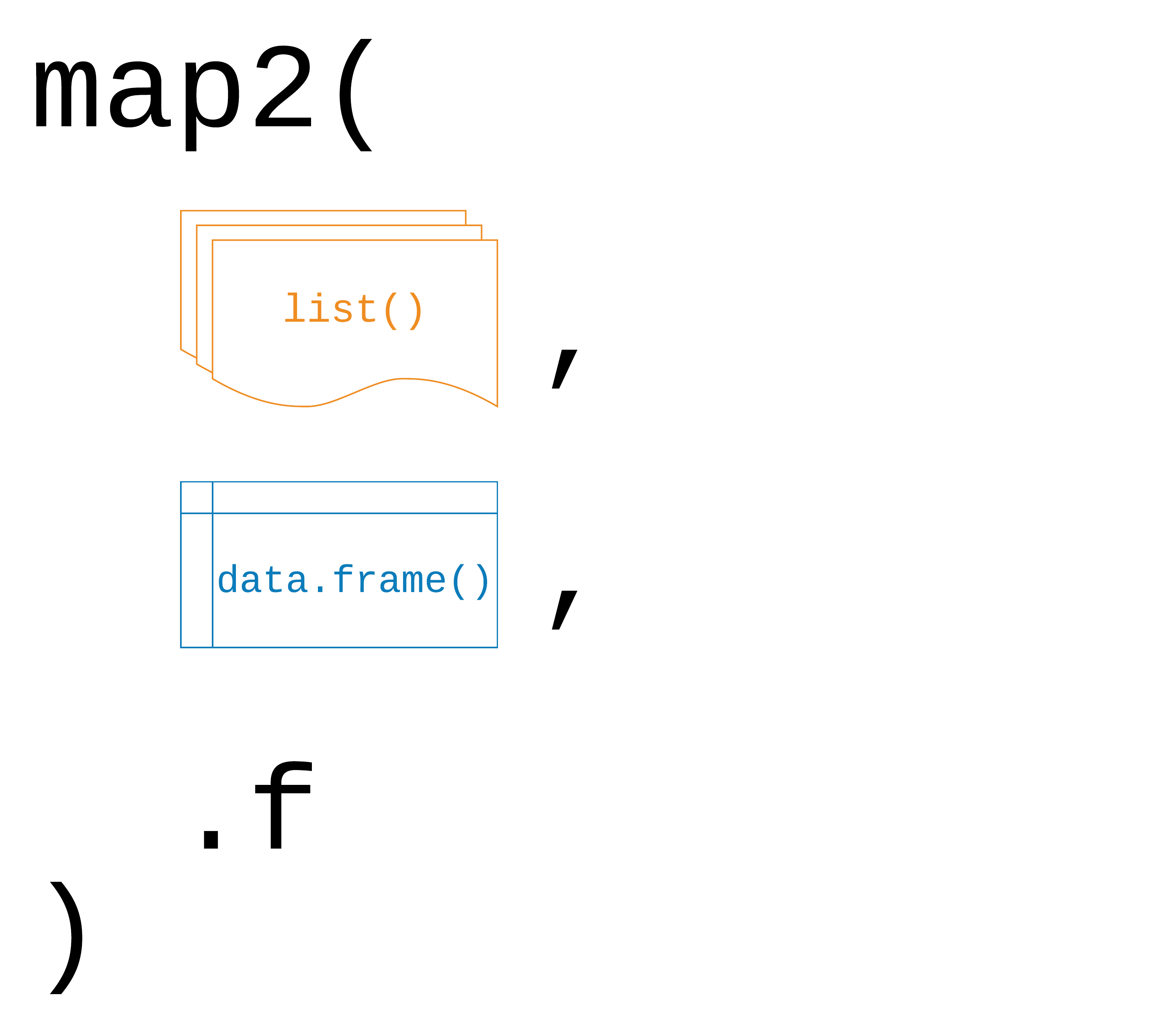
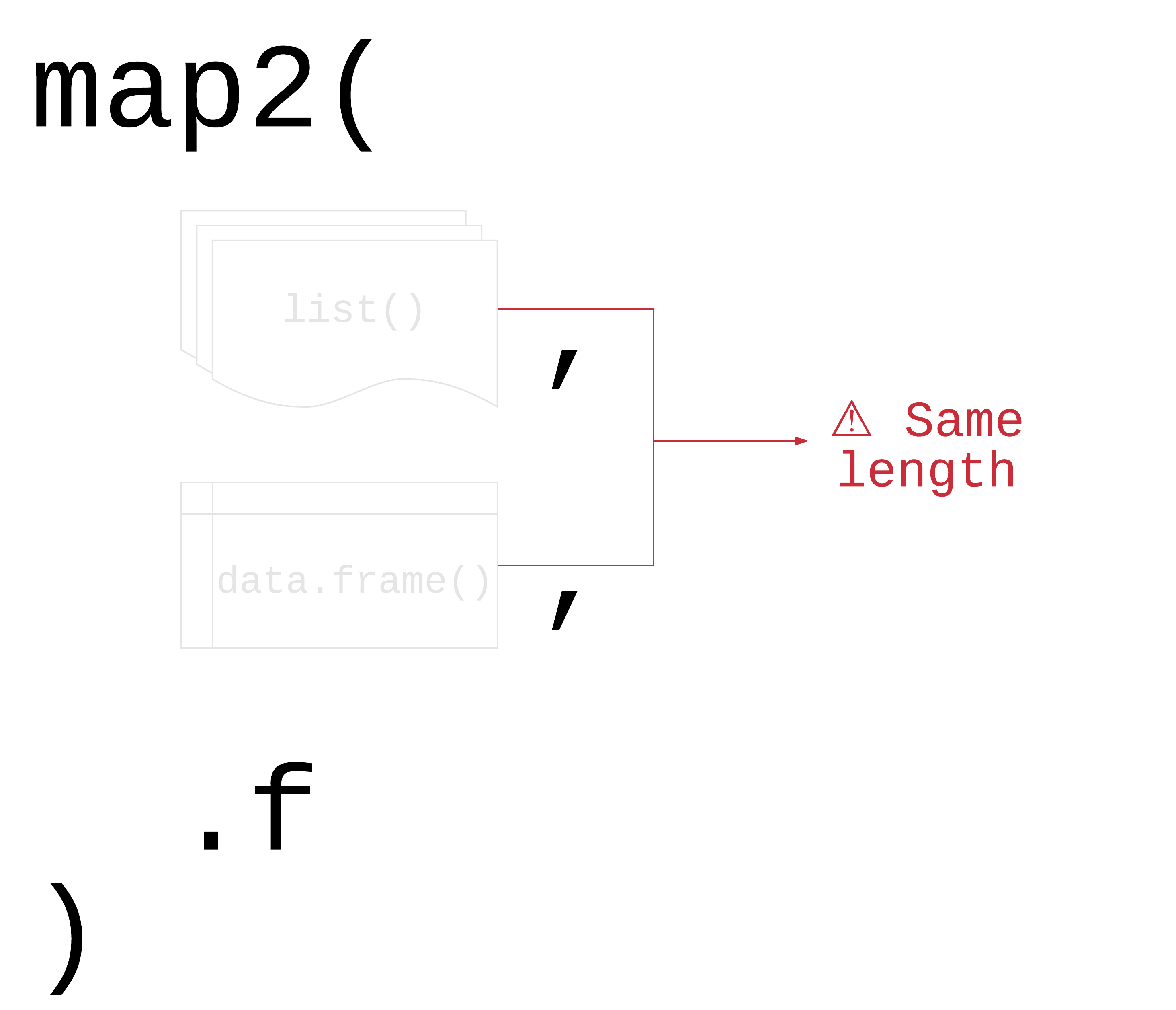
# BIC <dbl>, deviance <dbl>, df.residual <int>, …map2(.x, .y, .f)
.x, .y: a vector, list, or data frame
.f: a function that takes two arguments
Returns a list
map2()
[1] -3.0587804 1.4037210 -0.2195345 3.1492742Your Turn 9
Split the gapminder dataset into a list by country using the split() function
Create a list of models using map(). For the first argument, pass gapminder_countries. For the second, use the \() notation to write a model with lm(). Use lifeExp on the left hand side of the formula and year on the second. Pass .x to the data argument.
Use map2() to take the models list and the data set list and map them to predict(). Since we’re not adding new arguments, you don’t need to use \().
Your Turn 9
Your Turn 9
$Afghanistan
       1        2        3        4        5        6        7        8
29.90729 31.28394 32.66058 34.03722 35.41387 36.79051 38.16716 39.54380
       9       10       11       12
40.92044 42.29709 43.67373 45.05037

$Albania
       1        2        3        4        5        6        7        8
59.22913 60.90254 62.57596 64.24938 65.92279 67.59621 69.26962 70.94304
       9       10       11       12
72.61646 74.28987 75.96329 77.63671

$Algeria
       1        2        3        4        5        6        7        8
43.37497 46.22137 49.06777 51.91417 54.76057 57.60697 60.45337 63.29976
       9       10       11       12
66.14616 68.99256 71.83896 74.68536 | input 1 | input 2 | returns |
|---|---|---|
map() |
map2() |
list |
map_chr() |
map2_chr() |
character vector |
map_dbl() |
map2_dbl() |
double vector (numeric) |
map_int() |
map2_int() |
integer vector |
map_lgl() |
map2_lgl() |
logical vector |
map_dfc() |
map2_dfc() |
data frame (by column) |
map_dfr() |
map2_dfr() |
data frame (by row) |
Other mapping functions
pmap() and friends: take n lists or data frame with argument names
walk() and friends: for side effects like plotting; returns input invisibly
imap() and friends: includes counter i
map_if(), map_at(): Apply only to certain elements
| input 1 | input 2 | input n | returns |
|---|---|---|---|
map() |
map2() |
pmap() |
list |
map_chr() |
map2_chr() |
pmap_chr() |
character vector |
map_dbl() |
map2_dbl() |
pmap_dbl() |
double vector (numeric) |
map_int() |
map2_int() |
pmap_int() |
integer vector |
map_lgl() |
map2_lgl() |
pmap_lgl() |
logical vector |
map_dfc() |
map2_dfc() |
pmap_dfc() |
data frame (by column) |
map_dfr() |
map2_dfr() |
pmap_dfr() |
data frame (by row) |
walk() |
walk2() |
pwalk() |
input (side effects!) |
group_walk()
Use group_walk() for side effects across groups
group_walk()
temporary_folder
├── Africa.xlsx
├── Americas.xlsx
├── Asia.xlsx
├── Europe.xlsx
└── Oceania.xlsx
Your turn 10
Create a new directory using the fs package. Call it “figures”.
Write a function to plot a line plot of a given variable in gapminder over time, faceted by continent. Then, save the plot (how do you save a ggplot?). For the file name, paste together the folder, name of the variable, and extension so it follows the pattern "folder/variable_name.png"
Create a character vector that has the three variables we’ll plot: “lifeExp”, “pop”, and “gdpPercap”.
Use walk() to save a plot for each of the variables
Your turn 10
dir_create("figures")

ggsave_gapminder <- function(variable) {
  variable <- rlang::ensym(variable)
  p <- ggplot(
    gapminder,
    aes(x = year, y = {{ variable }}, color = country)
  ) +
    geom_line() +
    scale_color_manual(values = country_colors) +
    facet_wrap(~ continent) +
    theme(legend.position = "none")

  ggsave(
    filename = paste0("figures/", variable, ".png"),
    plot = p,
    dpi = 320
  )
}
Your turn 10
Base R
| base R | purrr |
|---|---|
lapply() |
map() |
vapply() |
map_*() |
sapply() |
? |
x[] <- lapply() |
map_dfc() |
mapply() |
map2(), pmap() |
Benefits of purrr
- Consistent
- Type-safe
Loops vs functional programming
Loops vs functional programming
Of course someone has to write loops. It doesn’t have to be you. —Jenny Bryan
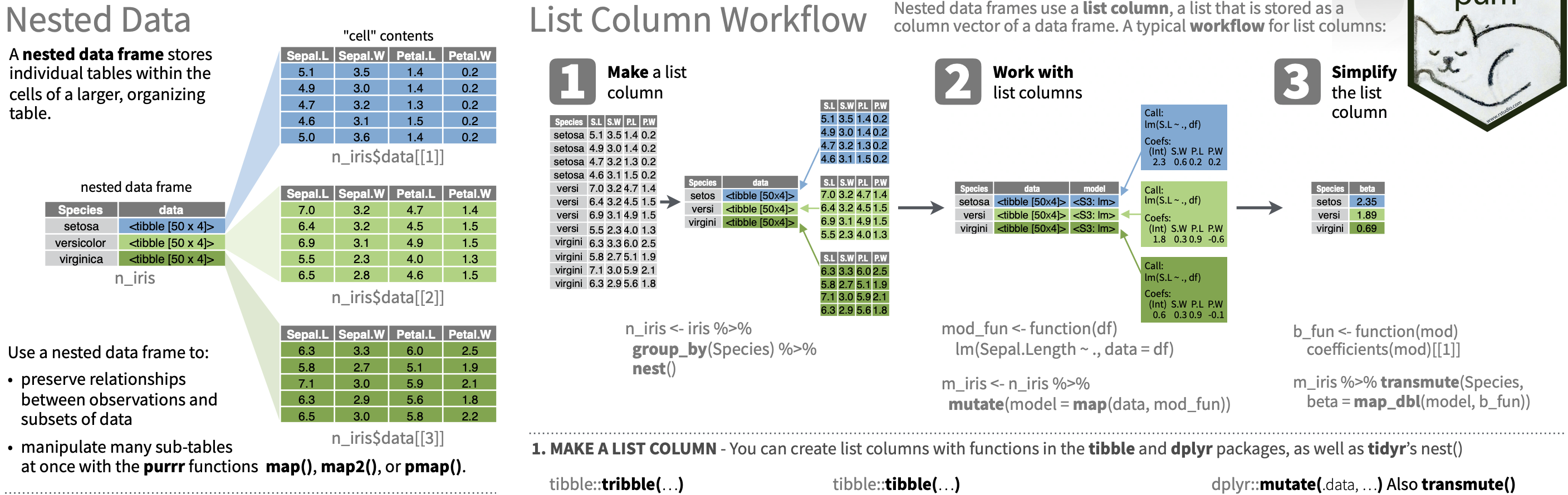
Working with lists and nested data
Working with lists and nested data
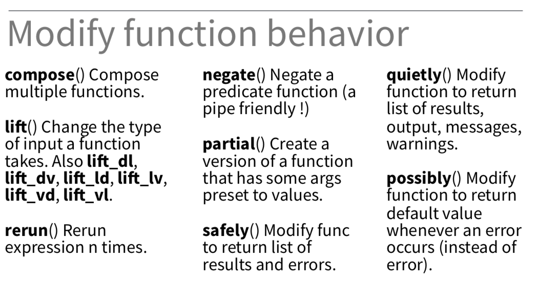
Adverbs: Modify function behavior