Tidying Data

tidyr

2025-08-09

tidyr

Functions for tidying data.

What is tidy data?

“Tidy datasets are all alike, but every messy dataset is messy in its own way.” — Hadley Wickham

Tidy Data

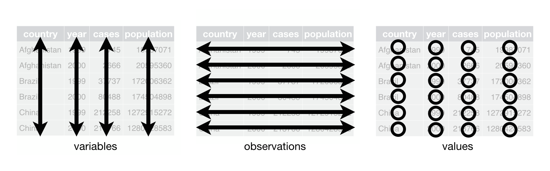
Each column is a single variable

Each row is a single observation

Each cell is a value

pivot_longer()

pivot_longer(<DATA>, <NAMES TO>, <VALUES TO>, <VARIABLES>)

Lord of the Rings

lotr <- tribble(
                         ~film,    ~race, ~female, ~male,
  "The Fellowship Of The Ring",    "Elf",   1229L,  971L,
  "The Fellowship Of The Ring", "Hobbit",     14L, 3644L,
  "The Fellowship Of The Ring",    "Man",      0L, 1995L,
              "The Two Towers",    "Elf",    331L,  513L,
              "The Two Towers", "Hobbit",      0L, 2463L,
              "The Two Towers",    "Man",    401L, 3589L,
      "The Return Of The King",    "Elf",    183L,  510L,
      "The Return Of The King", "Hobbit",      2L, 2673L,
      "The Return Of The King",    "Man",    268L, 2459L
)

Lord of the Rings

lotr

# A tibble: 9 × 4
  film                       race   female  male
  <chr>                      <chr>   <int> <int>
1 The Fellowship Of The Ring Elf      1229   971
2 The Fellowship Of The Ring Hobbit     14  3644
3 The Fellowship Of The Ring Man         0  1995
4 The Two Towers             Elf       331   513
5 The Two Towers             Hobbit      0  2463
6 The Two Towers             Man       401  3589
7 The Return Of The King     Elf       183   510
8 The Return Of The King     Hobbit      2  2673
9 The Return Of The King     Man       268  2459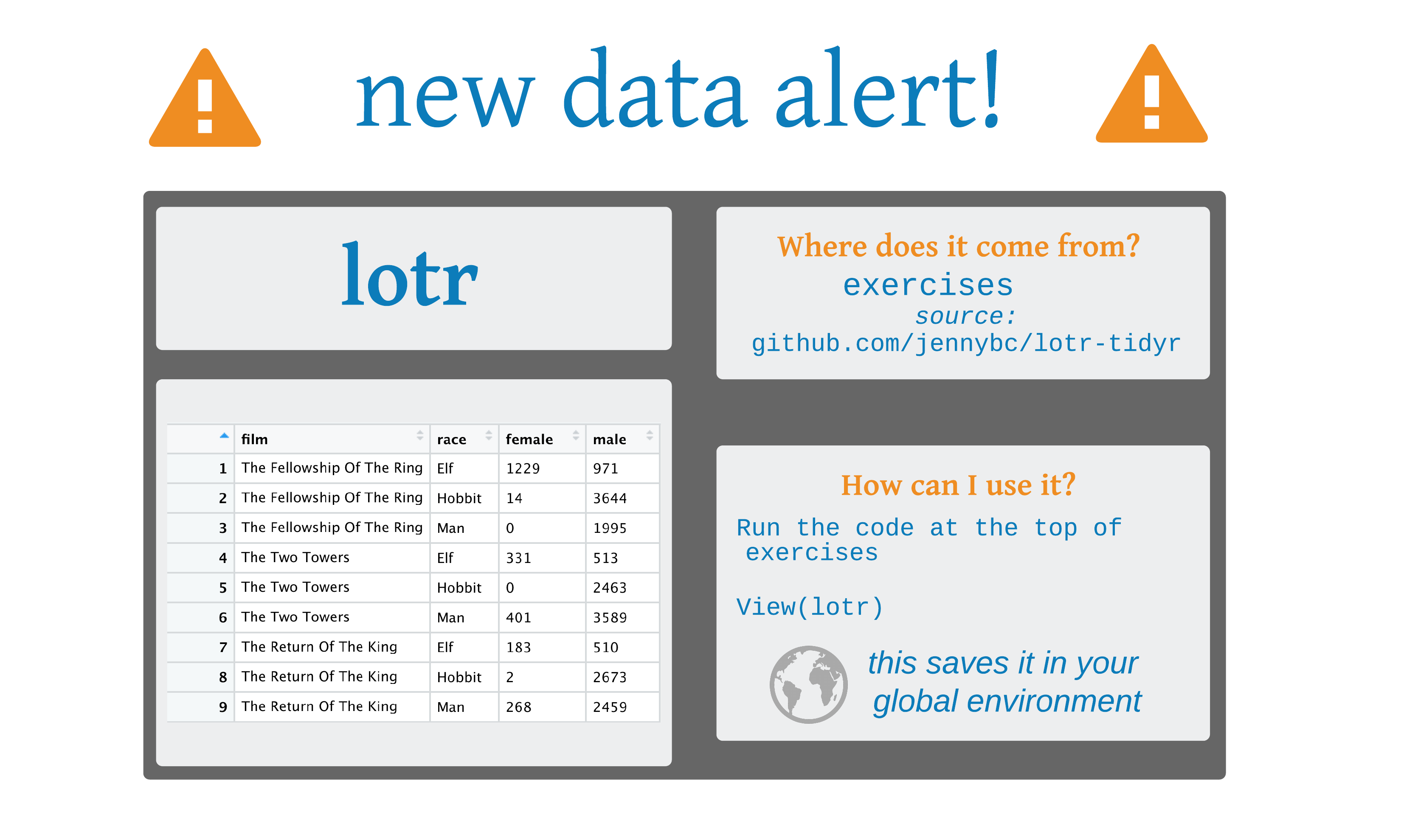

pivot_longer()

lotr |>
  pivot_longer(
    names_to = "sex",
    values_to = "words",
    cols = female:male
  )

pivot_longer()

# A tibble: 18 × 4
   film                       race   sex    words
   <chr>                      <chr>  <chr>  <int>
 1 The Fellowship Of The Ring Elf    female  1229
 2 The Fellowship Of The Ring Elf    male     971
 3 The Fellowship Of The Ring Hobbit female    14
 4 The Fellowship Of The Ring Hobbit male    3644
 5 The Fellowship Of The Ring Man    female     0
 6 The Fellowship Of The Ring Man    male    1995
 7 The Two Towers             Elf    female   331
 8 The Two Towers             Elf    male     513
 9 The Two Towers             Hobbit female     0
10 The Two Towers             Hobbit male    2463
11 The Two Towers             Man    female   401
12 The Two Towers             Man    male    3589
13 The Return Of The King     Elf    female   183
14 The Return Of The King     Elf    male     510
15 The Return Of The King     Hobbit female     2
16 The Return Of The King     Hobbit male    2673
17 The Return Of The King     Man    female   268
18 The Return Of The King     Man    male    2459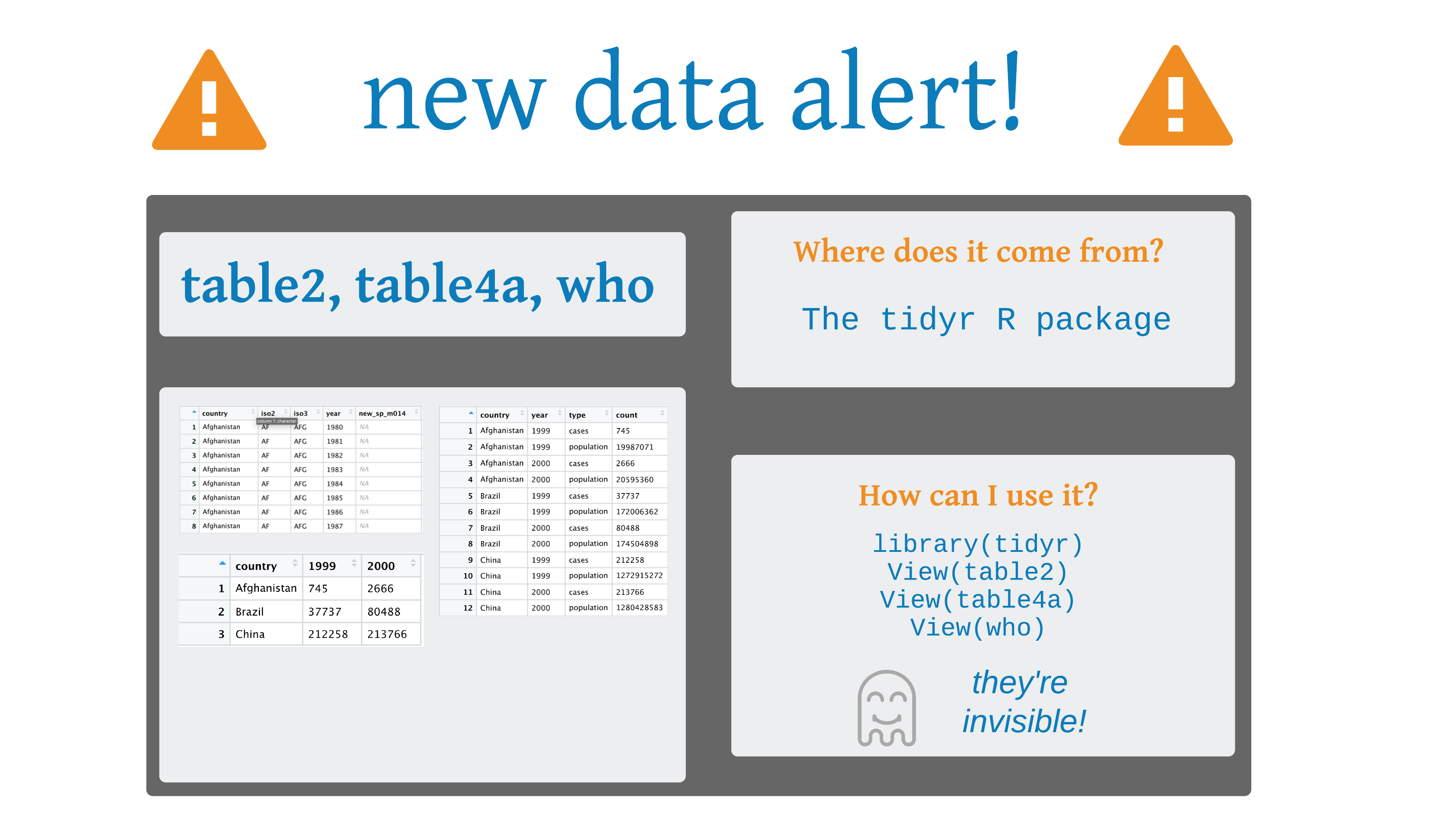

Your Turn 1

Use pivot_longer() to reorganize table4a into three columns: country, year, and cases.

Your Turn 1

table4a |>
  pivot_longer(
    names_to = "year",
    values_to = "cases",
    cols = -country
  )

# A tibble: 6 × 3
  country     year   cases
  <chr>       <chr>  <dbl>
1 Afghanistan 1999     745
2 Afghanistan 2000    2666
3 Brazil      1999   37737
4 Brazil      2000   80488
5 China       1999  212258
6 China       2000  213766

pivot_wider()

pivot_wider(<DATA>, <NAMES FROM>, <VALUES FROM>)

Animation by Mara Averick

pivot_wider()

lotr |>
  pivot_longer(
    names_to = "sex",
    values_to = "words",
    cols = female:male
  ) |>
  pivot_wider(
    names_from = race,
    values_from = words
  )

# A tibble: 6 × 5
  film                       sex      Elf Hobbit   Man
  <chr>                      <chr>  <int>  <int> <int>
1 The Fellowship Of The Ring female  1229     14     0
2 The Fellowship Of The Ring male     971   3644  1995
3 The Two Towers             female   331      0   401
4 The Two Towers             male     513   2463  3589
5 The Return Of The King     female   183      2   268
6 The Return Of The King     male     510   2673  2459

Your Turn 2

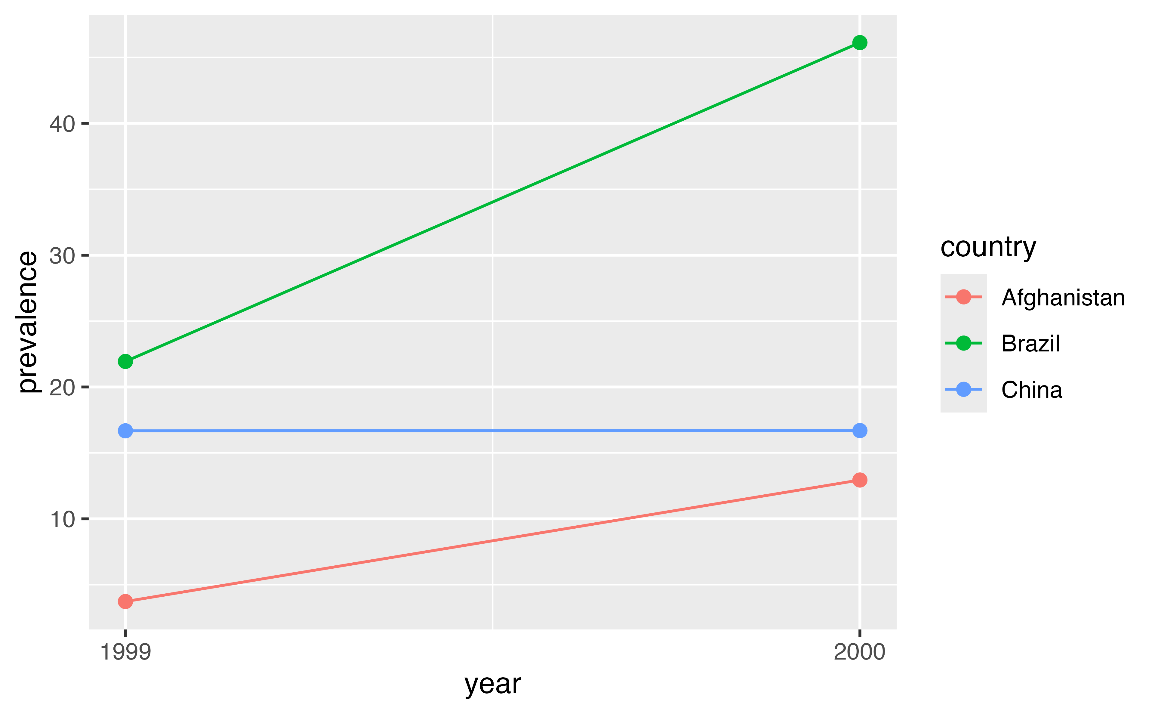
Use pivot_wider() to reorganize table2 into four columns: country, year, cases, and population.

Create a new variable called prevalence that divides cases by population multiplied by 100000.

Pass the data frame to a ggplot. Make a scatter plot with year on the x axis and prevalence on the y axis. Set the color aesthetic (aes()) to country. Use size = 2 for the points. Add a line geom.

table2

Your Turn 2

table2 |>
  pivot_wider(
    names_from = type,
    values_from = count
  ) |>
  mutate(prevalence = (cases / population) * 100000)

# A tibble: 6 × 5
  country      year  cases population prevalence
  <chr>       <dbl>  <dbl>      <dbl>      <dbl>
1 Afghanistan  1999    745   19987071       3.73
2 Afghanistan  2000   2666   20595360      12.9 
3 Brazil       1999  37737  172006362      21.9 
4 Brazil       2000  80488  174504898      46.1 
5 China        1999 212258 1272915272      16.7 
6 China        2000 213766 1280428583      16.7 

Your Turn 2

table2 |>
  pivot_wider(
    names_from = type,
    values_from = count
  ) |>
  mutate(prevalence = (cases / population) * 100000) |>
  ggplot(aes(x = year, y = prevalence, color = country)) +
  geom_point(size = 2) +
  geom_line() +
  scale_x_continuous(breaks = c(1999L, 2000L))

Your Turn 2

Your Turn 3

Pivot the 5th through 60th columns of who so that the names of the columns go into a new variable called codes and the values go into a new variable called n. Then select just the country, year, codes and n variables.

who

Your Turn 3

who |>
  pivot_longer(
    names_to = "codes",
    values_to = "n",
    cols = 5:60
  ) |>
  select(country, year, codes, n)

Your Turn 3

# A tibble: 405,440 × 4
   country      year codes            n
   <chr>       <dbl> <chr>        <dbl>
 1 Afghanistan  1980 new_sp_m014     NA
 2 Afghanistan  1980 new_sp_m1524    NA
 3 Afghanistan  1980 new_sp_m2534    NA
 4 Afghanistan  1980 new_sp_m3544    NA
 5 Afghanistan  1980 new_sp_m4554    NA
 6 Afghanistan  1980 new_sp_m5564    NA
 7 Afghanistan  1980 new_sp_m65      NA
 8 Afghanistan  1980 new_sp_f014     NA
 9 Afghanistan  1980 new_sp_f1524    NA
10 Afghanistan  1980 new_sp_f2534    NA
# ℹ 405,430 more rows

separate()/unite()

separate(
  <DATA>,
  <VARIABLE>,
  into = c("<VARIABLE1>", "<VARIABLE2>")
)

unite(<DATA>, <VARIABLES>)

Your Turn 4

Use the cases data below. Separate the sex_age column into sex and age columns.

cases <- tribble(
   ~id,     ~sex_age,
   "1",    "male_56",
   "2",  "female_77",
   "3",  "female_49"
)
separate(_______, _______, into = c("_______", "_______"))

Your Turn 4

cases <- tribble(
   ~id,     ~sex_age,
   "1",    "male_56",
   "2",  "female_77",
   "3",  "female_49"
)
separate(cases, sex_age, into = c("sex", "age"))

# A tibble: 3 × 3
  id    sex    age  
  <chr> <chr>  <chr>
1 1     male   56   
2 2     female 77   
3 3     female 49   

Your Turn 4

cases <- tribble(
   ~id,     ~sex_age,
   "1",    "male_56",
   "2",  "female_77",
   "3",  "female_49"
)
separate(
  cases,
  sex_age,
  into = c("sex", "age"),
  convert = TRUE
)

# A tibble: 3 × 3
  id    sex      age
  <chr> <chr>  <int>
1 1     male      56
2 2     female    77
3 3     female    49

Your Turn 5: Challenge!

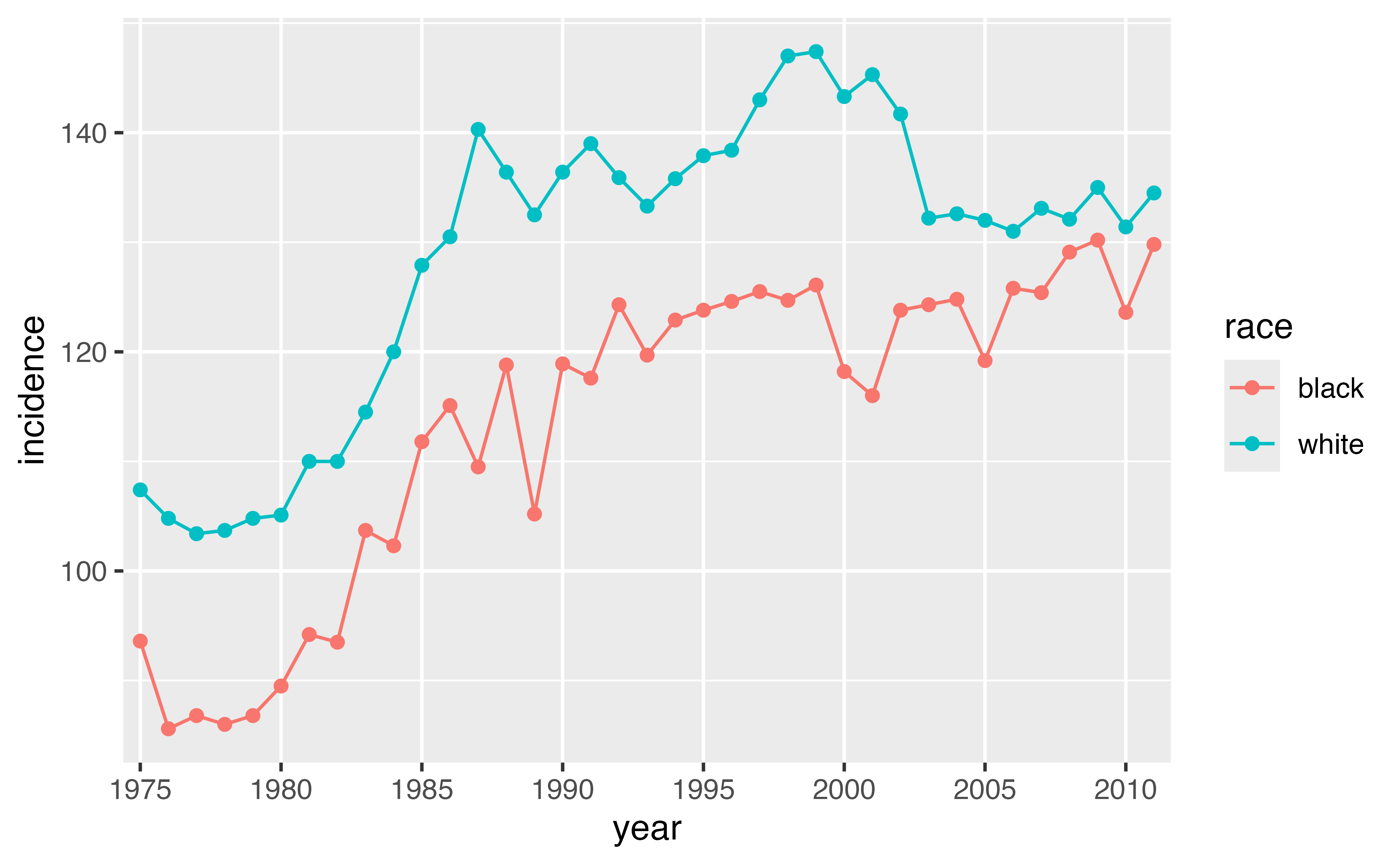
There are two CSV files in this folder containing SEER data in breast cancer incidence in white and black women. For both sets of data:

Import the data

Pivot the columns into 2 new columns called year and incidence

Add a new variable called race. Remember that each data set corresponds to a single race.

Bind the data sets together using bind_rows() from the dplyr package. Either save it as a new object or pipe the result directly into the ggplot2 code.

Plot the data using the code below. Fill in the blanks to have year on the x-axis, incidence on the y-axis, and race as the color aesthetic.

Your Turn 5: No solution 😈

Other neat tidyr tools

Uncounting frequency tables

lotr |>
  pivot_longer(
    names_to = "sex",
    values_to = "count",
    cols = c(female, male)
  ) |>
  uncount(count)

Other neat tidyr tools

# A tibble: 21,245 × 3
   film                       race  sex   
   <chr>                      <chr> <chr> 
 1 The Fellowship Of The Ring Elf   female
 2 The Fellowship Of The Ring Elf   female
 3 The Fellowship Of The Ring Elf   female
 4 The Fellowship Of The Ring Elf   female
 5 The Fellowship Of The Ring Elf   female
 6 The Fellowship Of The Ring Elf   female
 7 The Fellowship Of The Ring Elf   female
 8 The Fellowship Of The Ring Elf   female
 9 The Fellowship Of The Ring Elf   female
10 The Fellowship Of The Ring Elf   female
# ℹ 21,235 more rows

Other neat tidyr tools

Work with data frames

crossing() and expand()

nest() and unnest()

Other neat tidyr tools

Work with missing data

complete()

drop_na() and replace_na()

Resources

R for Data Science: A comprehensive but friendly introduction to the tidyverse. Free online.

Posit Recipes: Common code patterns in R (with some comparisons to SAS)