Types, vectors, and functions in R

2025-08-09

Vectors and Types

Vectors

c(1, 3, 5)

c(TRUE, FALSE, TRUE, TRUE)

c("red", "blue")

Vectors

Vectors have 1 dimension

Vectors have a length

length(c("blue", "red"))

[1] 2

Some vectors have names.

names(c("x" = 1, "y" = 1))

[1] "x" "y"

Vectors have types and classes

class(c("blue", "red"))

[1] "character"

Types

Numeric/double (c(1.0, 2.0, 3.0))

Integer (c(1L, 2L, 3L))

Character (c("a", "b", "c"))

Factor (factor(c("a", "b", "c")))

Logical (TRUE)

Dates and times

Packages to work with types and classes

Strings/character: stringr

Factors: forcats

Dates: lubridate

Making vectors

1:3

[1] 1 2 3

c(1, 2, 3)

[1] 1 2 3

rep(1, 3)

[1] 1 1 1

seq(from = 1, to = 3, by = .5)

[1] 1.0 1.5 2.0 2.5 3.0

Your Turn 1

Create a character vector of colors using c(). Use the colors "grey90" and "steelblue". Assign the vector to a name.

Use the vector you just created to change the colors in the plot below using scale_color_manual(). Pass it using the values argument.

Your Turn 1

cols <- c("grey90", "steelblue") 

gapminder |> 
  mutate(rwanda = country == "Rwanda") |> 
  ggplot(aes(year, lifeExp, color = rwanda, group = country)) + 
  geom_line() +
  scale_color_manual(values = cols) +  
  theme_minimal()

Your Turn 1

Working with vectors

Subset vectors with [] or [[]]

x <- c(1, 5, 7)
x[2]

[1] 5

x[[2]]

[1] 5

x[c(FALSE, TRUE, FALSE)]

[1] 5

x[[c(FALSE, TRUE, FALSE)]]

Error in x[[c(FALSE, TRUE, FALSE)]]: attempt to select more than one element in vectorIndex

Working with vectors

Modify elements

x

[1] 1 5 7

Working with vectors

Modify elements

x[[2]] <- 100
x

[1]   1 100   7

Working with vectors

Modify elements

x[x > 10] <- NA
x

[1]  1 NA  7

cols <- c("grey90", "steelblue") 

gapminder |> 
  mutate(rwanda = ifelse(country == "Rwanda", TRUE, FALSE)) |> 
  ggplot(aes(year, lifeExp, color = rwanda, group = country)) + 
  geom_line() +
  scale_color_manual(values = cols) +  
  theme_minimal()

cols <- c("grey90", "steelblue") 

gapminder |> 
  mutate(rwanda = ifelse(country == "Rwanda", TRUE, FALSE)) |> 
  ggplot(aes(year, lifeExp, group = country)) +
  geom_line( 
    data = function(x) filter(x, !rwanda), 
    color = cols[[1]]
  ) + 
  theme_minimal()

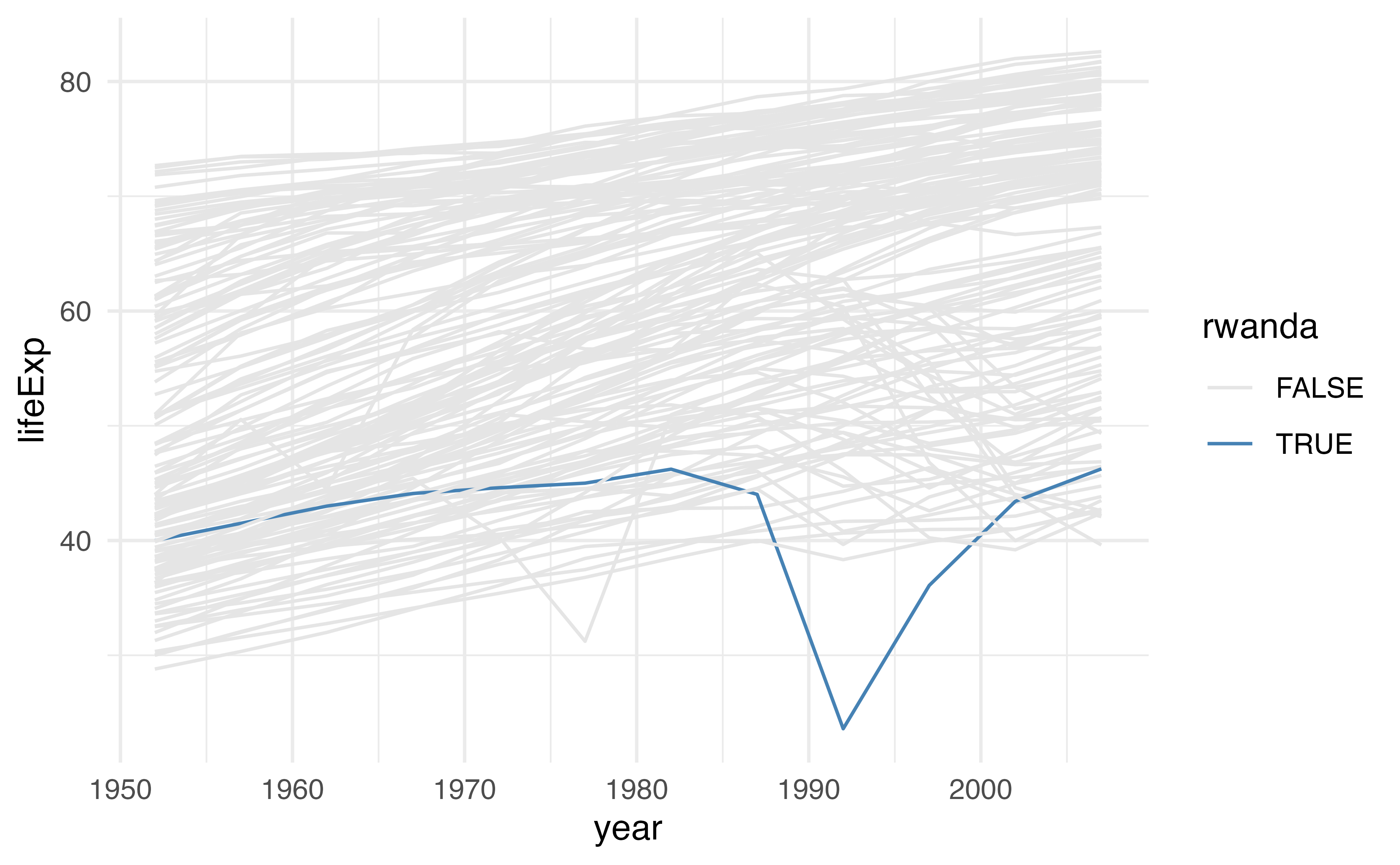
cols <- c("grey90", "steelblue") 

gapminder |> 
  mutate(rwanda = ifelse(country == "Rwanda", TRUE, FALSE)) |> 
  ggplot(aes(year, lifeExp, color = rwanda, group = country)) + 
  geom_line(
    data = function(x) filter(x, !rwanda), 
    color = cols[[1]]
  ) +
  geom_line(
    data = function(x) filter(x, rwanda), 
    color = cols[[2]], 
    linewidth = 1.5 
  ) + 
  theme_minimal()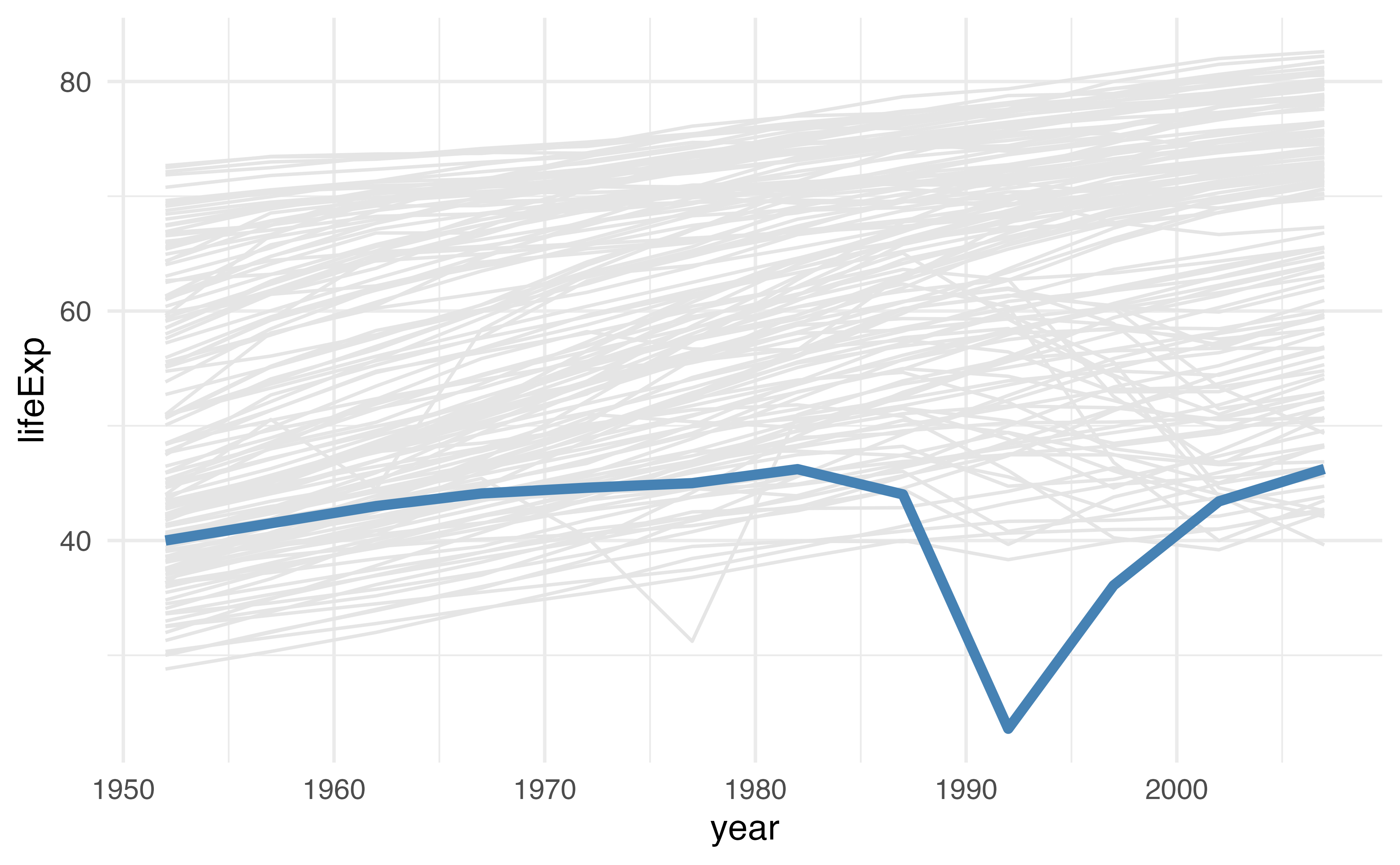

Your Turn 2

Create a numeric vector that has the following values: 3, 5, NA, 2, and NA.

Try using sum(). Then add na.rm = TRUE.

Check which values are missing with is.na(); save the results to a new object and take a look

Change all missing values of x to -9999.

Try sum() again without na.rm = TRUE.

Your Turn 2

x <- c(3, 5, NA, 2, NA)
sum(x)

[1] NA

Your Turn 2

sum(x, na.rm = TRUE)

[1] 10

Your Turn 2

x_missing <- is.na(x)
x_missing

[1] FALSE FALSE  TRUE FALSE  TRUE

x[x_missing] <- -9999
x

[1]     3     5 -9999     2 -9999

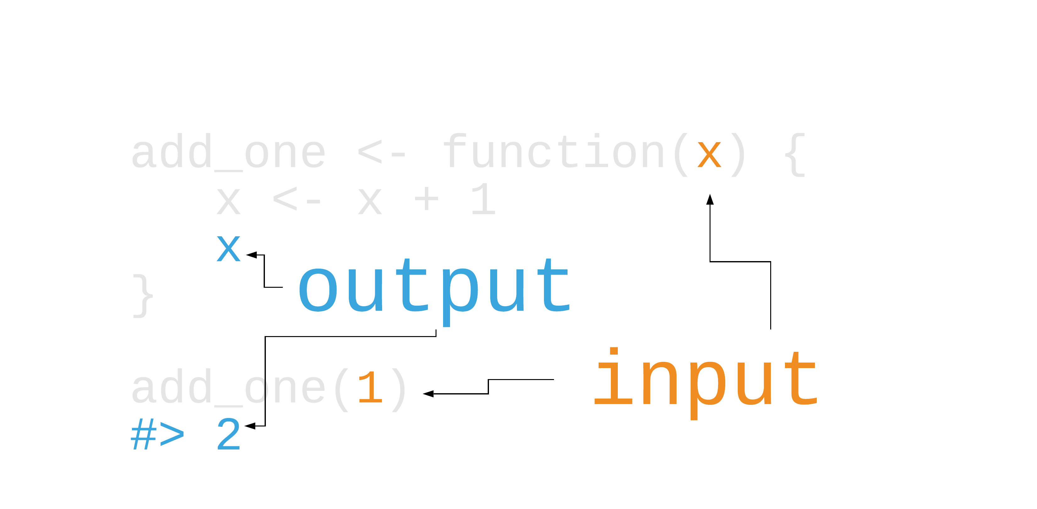
Writing Functions

Functions that return vectors

gdpPercap <- gapminder |> 
  filter(year == 1952, continent == "Americas") |> 
  pull(gdpPercap)

sum(gdpPercap)

[1] 101976.6

Functions that return data frames

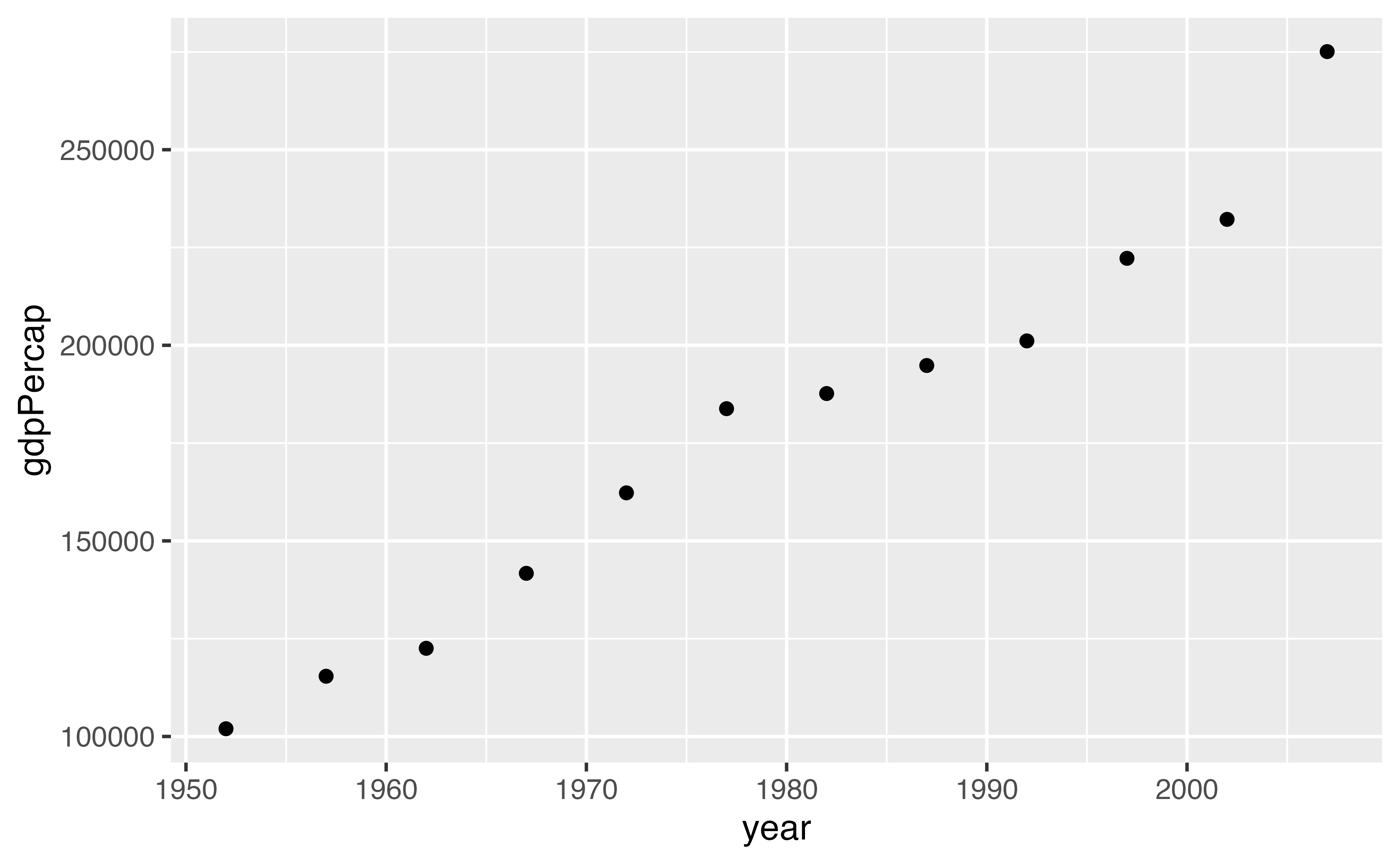
gapminder |> 
  group_by(year) |> 
  filter(continent == "Americas") |> 
  summarize(gdpPercap = sum(gdpPercap))

# A tibble: 12 × 2
    year gdpPercap
   <int>     <dbl>
 1  1952   101977.
 2  1957   115401.
 3  1962   122539.
 4  1967   141706.
 5  1972   162283.
 6  1977   183800.
 7  1982   187668.
 8  1987   194835.
 9  1992   201123.
10  1997   222233.
11  2002   232192.
12  2007   275076.

Functions that make plots

gapminder |> 
  group_by(year) |> 
  filter(continent == "Americas") |> 
  summarize(gdpPercap = sum(gdpPercap)) |> 
  ggplot(aes(year, gdpPercap)) +
  geom_point()

Why write functions?

To make repetitive code reusable

To make complex code understandable

To make useful code shareable

Writing functions

Writing functions

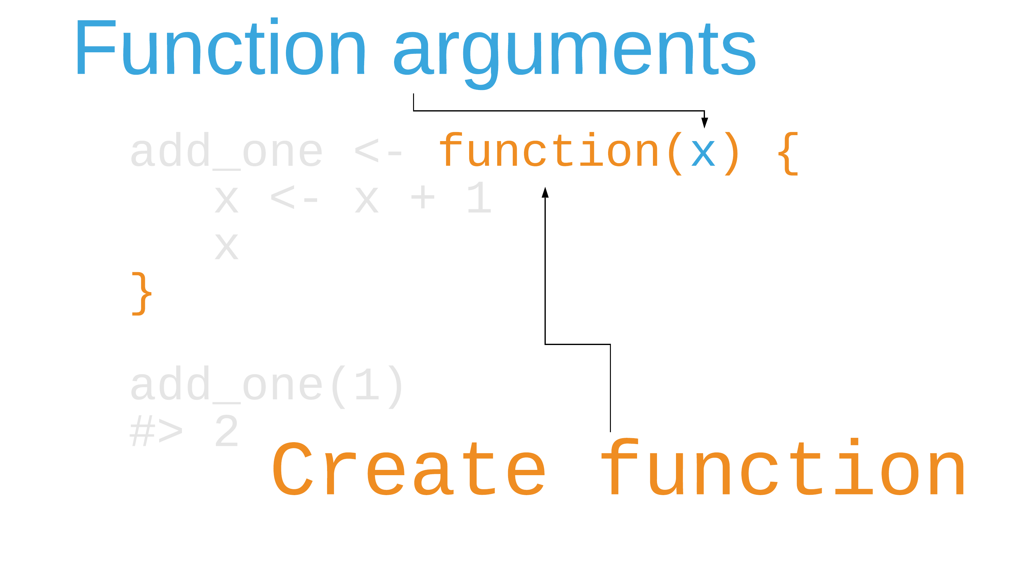
Writing functions

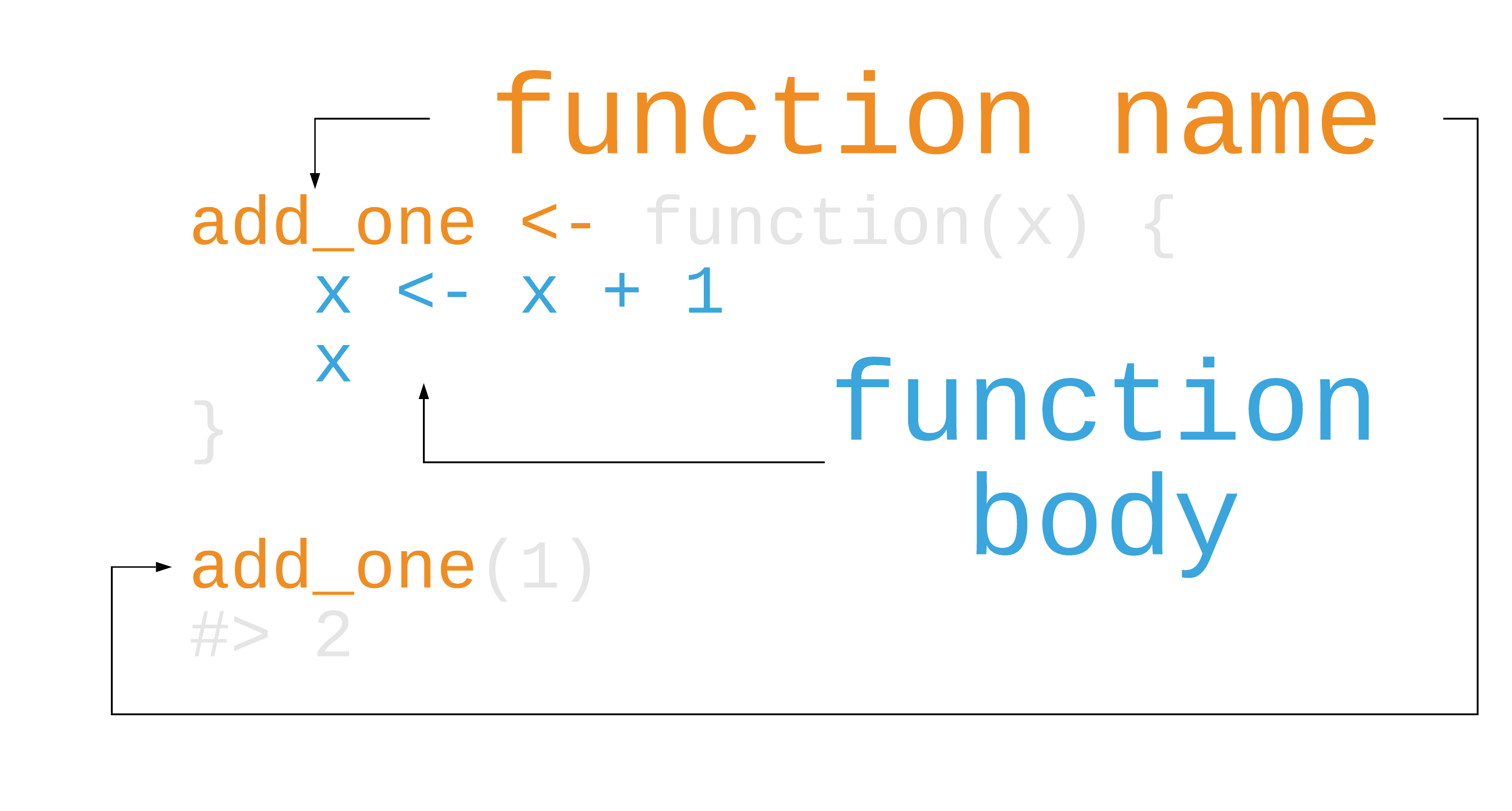
Writing functions

Your Turn 3

Create a function called sim_data that doesn’t take any arguments.

In the function body, we’ll return a tibble.

For x, have rnorm() return 50 random numbers.

For sex, use rep() to create 50 values of “male” and “female”. Hint: You’ll have to give rep() a character vector for the first argument. The times argument is how many times rep() should repeat the first argument, so make sure you account for that.

For age use the sample() function to sample 50 numbers from 25 to 50 with replacement.

Call sim_data()

Your Turn 3

sim_data <- function() {
  tibble(
    x = rnorm(50), 
    sex = rep(c("male", "female"), times = 25),
    age = sample(25:50, size = 50, replace = TRUE)
  )
}

sim_data()

Your Turn 3

# A tibble: 50 × 3
         x sex      age
     <dbl> <chr>  <int>
 1  0.0332 male      28
 2  2.31   female    42
 3 -0.589  male      32
 4  0.734  female    43
 5  0.489  male      28
 6  0.493  female    45
 7 -0.342  male      46
 8  0.861  female    50
 9  1.06   male      29
10 -0.916  female    45
# ℹ 40 more rows

E-Values

The strength of unmeasured confounding required to explain away a value

Rate ratio: 3.9 = E-value: 7.3

Your Turn 4

Write a function to calculate an E-Value given an RR.

Call the function evalue and give it an argument called estimate. In the body of the function, calculate the E-Value using estimate + sqrt(estimate * (estimate - 1))

Call evalue() for a risk ratio of 3.9

Your Turn 4

evalue <- function(estimate) {
  estimate + sqrt(estimate * (estimate - 1))
}

Invoking the function with ()

evalue(3.9)

[1] 7.263034

Control Flow

if (PREDICATE) {
  do_something()
}

Control Flow

if (PREDICATE) {
  do_something()
} else {
  do_something_for_everything_else()
}

Control Flow

if (PREDICATE) {
  do_something()
} else if (ANOTHER_PREDICATE) {
  do_something_else()
} else  {
  do_something_for_everything_else()
}

Make a prediction

What will y be?

x <- 99
if (x < 10) {
  y <- "a"
} else if (is.na(x)) {
  y <- NA
} else  {
  y <- "z"
}

y

[1] "z"

If statements are for a single TRUE or FALSE

x <- rnorm(100)
if (x > 0) {
  x + 1
}

Error in if (x > 0) {: the condition has length > 1

Conditional values with vectors

ifelse(PREDICATE_VECTOR, true_result, false_result)
dplyr::case_when(
  PREDICATE_VECTOR ~ true_result,
  PREDICATE_VECTOR ~ next_true_result, 
  .default = default_result
)
# also see `switch()`

Conditional values with vectors

x <- -2:2
ifelse(x >= 0, "positive", "negative")

[1] "negative" "negative" "positive" "positive" "positive"

If-else with vectors

case_when(
  x > 0 ~ "positive", 
  x == 0 ~ "zero",
  .default = "negative"
)

[1] "negative" "negative" "zero"     "positive" "positive"

Validation and stopping

if (is.numeric(x)) stop(), warn()

function(x) {
  if (is.numeric(x)) stop("x must be a character")
  # do something with a character
}

Your Turn 5

Use if () together with is.numeric() to make sure estimate is a number. Remember to use ! for not.

If the estimate is less than 1, set estimate to be equal to 1 / estimate.

Call evalue() for a risk ratio of 3.9. Then try 0.80. Then try a character value.

Your Turn 5

evalue <- function(estimate) { 
  if (!is.numeric(estimate)) stop("`estimate` must be numeric")
  if (estimate < 1) estimate <- 1 / estimate
  estimate + sqrt(estimate * (estimate - 1))
}

Your Turn 5

evalue(3.9)

[1] 7.263034

evalue(.80)

[1] 1.809017

evalue("3.9")

Error in evalue("3.9"): `estimate` must be numeric

Your Turn 6

Add a new argument called type. Set the default value to "rr"

Check if type is equal to "or". If it is, set the value of estimate to be sqrt(estimate)

Call evalue() for a risk ratio of 3.9. Then try it again with type = "or".

Your Turn 6

evalue <- function(estimate, type = "rr") {
  if (!is.numeric(estimate)) stop("`estimate` must be numeric")
  if (type == "or") estimate <- sqrt(estimate)
  if (estimate < 1) estimate <- 1 / estimate
  estimate + sqrt(estimate * (estimate - 1))
}

Your Turn 6

evalue(3.9)

[1] 7.263034

evalue(3.9, type = "or")

[1] 3.362342

Your Turn 7: Challenge!

Create a new function called transform_to_rr with arguments estimate and type.

Use the same code above to check if type == "or" and transform if so. Add another line that checks if type == "hr". If it does, transform the estimate using this formula: (1 - 0.5^sqrt(estimate)) / (1 - 0.5^sqrt(1 / estimate)).

Move the code that checks if estimate < 1 to transform_to_rr (below the OR and HR transformations)

Return estimate

In evalue(), change the default argument of type to be a character vector containing “rr”, “or”, and “hr”.

Get and validate the value of type using match.arg(). Follow the pattern argument_name <- match.arg(argument_name)

Transform estimate using transform_to_rr(). Don’t forget to pass it both estimate and type!

Your Turn 7: Challenge!

transform_to_rr <- function(estimate, type) {
  if (type == "or") estimate <- sqrt(estimate)
  if (type == "hr") { 
    estimate <- 
      (1 - 0.5^sqrt(estimate)) / (1 - 0.5^sqrt(1 / estimate)) 
  } 
  if (estimate < 1) estimate <- 1 / estimate
  
  estimate
}

evalue <- function(estimate, type = c("rr", "or", "hr")) {
  # validate arguments
  if (!is.numeric(estimate)) stop("`estimate` must be numeric")
  type <- match.arg(type) 
  
  # calculate evalue
  estimate <- transform_to_rr(estimate, type) 
  estimate + sqrt(estimate * (estimate - 1))
}

Your Turn 7: Challenge!

evalue(3.9)

[1] 7.263034

evalue(3.9, type = "or")

[1] 3.362342

evalue(3.9, type = "hr")

[1] 4.474815

evalue(3.9, type = "rd")

Error in match.arg(type): 'arg' should be one of "rr", "or", "hr"

Programming with the tidyverse

Pass the dots: ...

select_gapminder <- function(...) {
  gapminder |> 
    select(...) 
}

select_gapminder(pop, year)

Pass the dots: ...

# A tibble: 1,704 × 2
        pop  year
      <int> <int>
 1  8425333  1952
 2  9240934  1957
 3 10267083  1962
 4 11537966  1967
 5 13079460  1972
 6 14880372  1977
 7 12881816  1982
 8 13867957  1987
 9 16317921  1992
10 22227415  1997
# ℹ 1,694 more rows

Your Turn 8

Use ... to pass the arguments of your function, filter_summarize(), to filter().

In summarize, get the n and mean life expectancy for the data set

Check filter_summarize() with year == 1952.

Try filter_summarize() again for 2002, but also filter countries that have the word ” and ” in the country name (e.g., it should detect “Trinidad and Tobago” but not “Iceland”). Use str_detect() from the stringr package.

Your Turn 8

filter_summarize <- function(...) { 
  gapminder |> 
    filter(...) |> 
    summarize(n = n(), mean_lifeExp = mean(lifeExp))
}

filter_summarize(year == 1952)

# A tibble: 1 × 2
      n mean_lifeExp
  <int>        <dbl>
1   142         49.1

filter_summarize(year == 2002, str_detect(country, " and "))

# A tibble: 1 × 2
      n mean_lifeExp
  <int>        <dbl>
1     4         69.9

Writing functions with dplyr, ggplot2, and friends

plot_hist <- function(x) {
  ggplot(gapminder, aes(x = x)) + geom_histogram()
}

plot_hist(lifeExp)

Error in `geom_histogram()`:
! Problem while computing aesthetics.
ℹ Error occurred in the 1st layer.
Caused by error:
! object 'lifeExp' not found

Programming with dplyr, ggplot2, and friends

plot_hist <- function(x) {
  ggplot(gapminder, aes(x = x)) + geom_histogram()
}

plot_hist("lifeExp")

Error in `geom_histogram()`:
! Problem while computing stat.
ℹ Error occurred in the 1st layer.
Caused by error in `setup_params()`:
! `stat_bin()` requires a continuous x aesthetic.
✖ the x aesthetic is discrete.
ℹ Perhaps you want `stat="count"`?

Curly-curly: {{ variable }}

plot_hist <- function(x) {
  ggplot(gapminder, aes(x = {{ x }})) + geom_histogram()
}

plot_hist(lifeExp)

Your turn 9

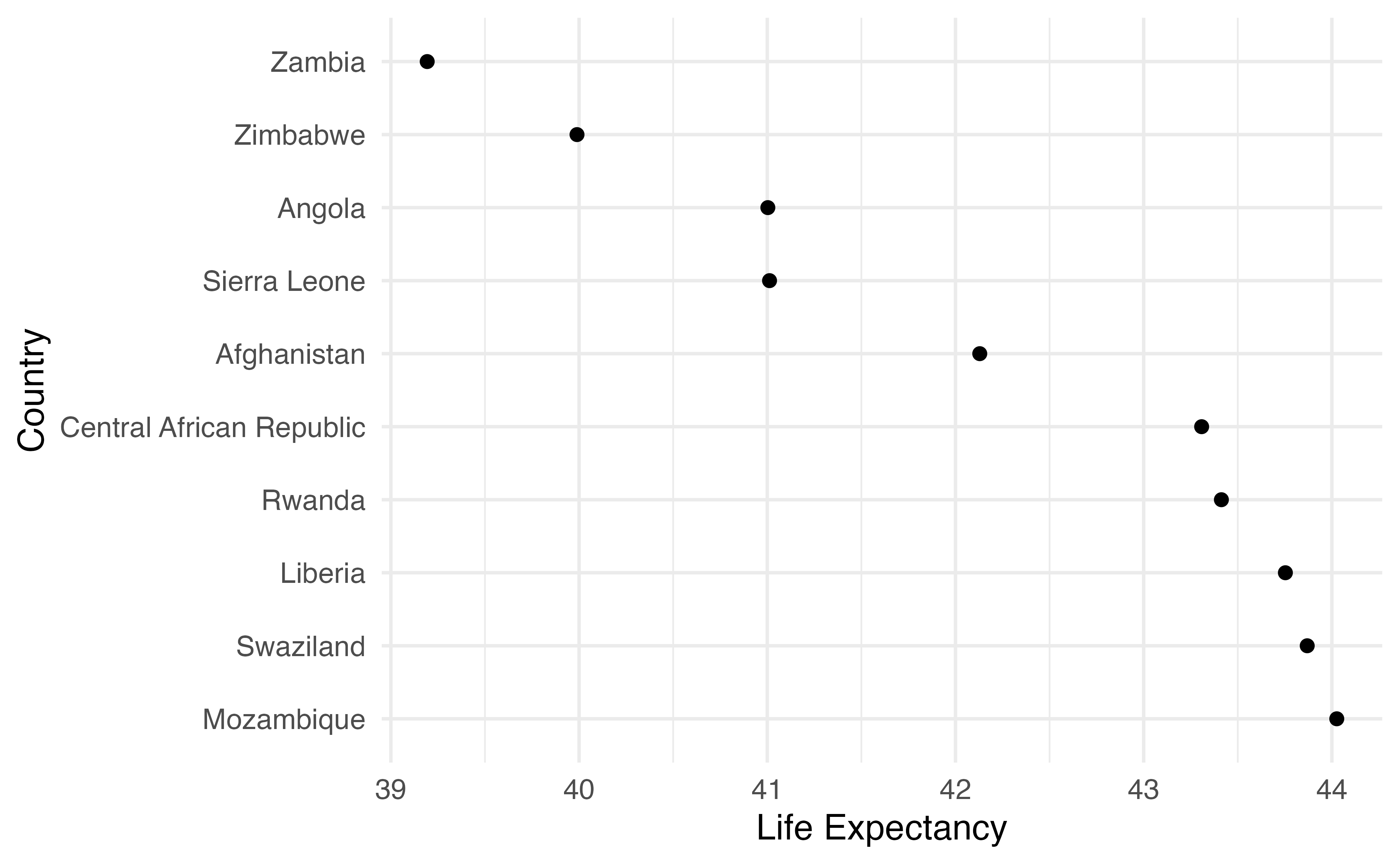
Filter gapminder by year using the value of .year (notice the period before hand!). You do NOT need curly-curly for this. (Why is that?)

Arrange it by the variable. This time, do wrap it in curly-curly!

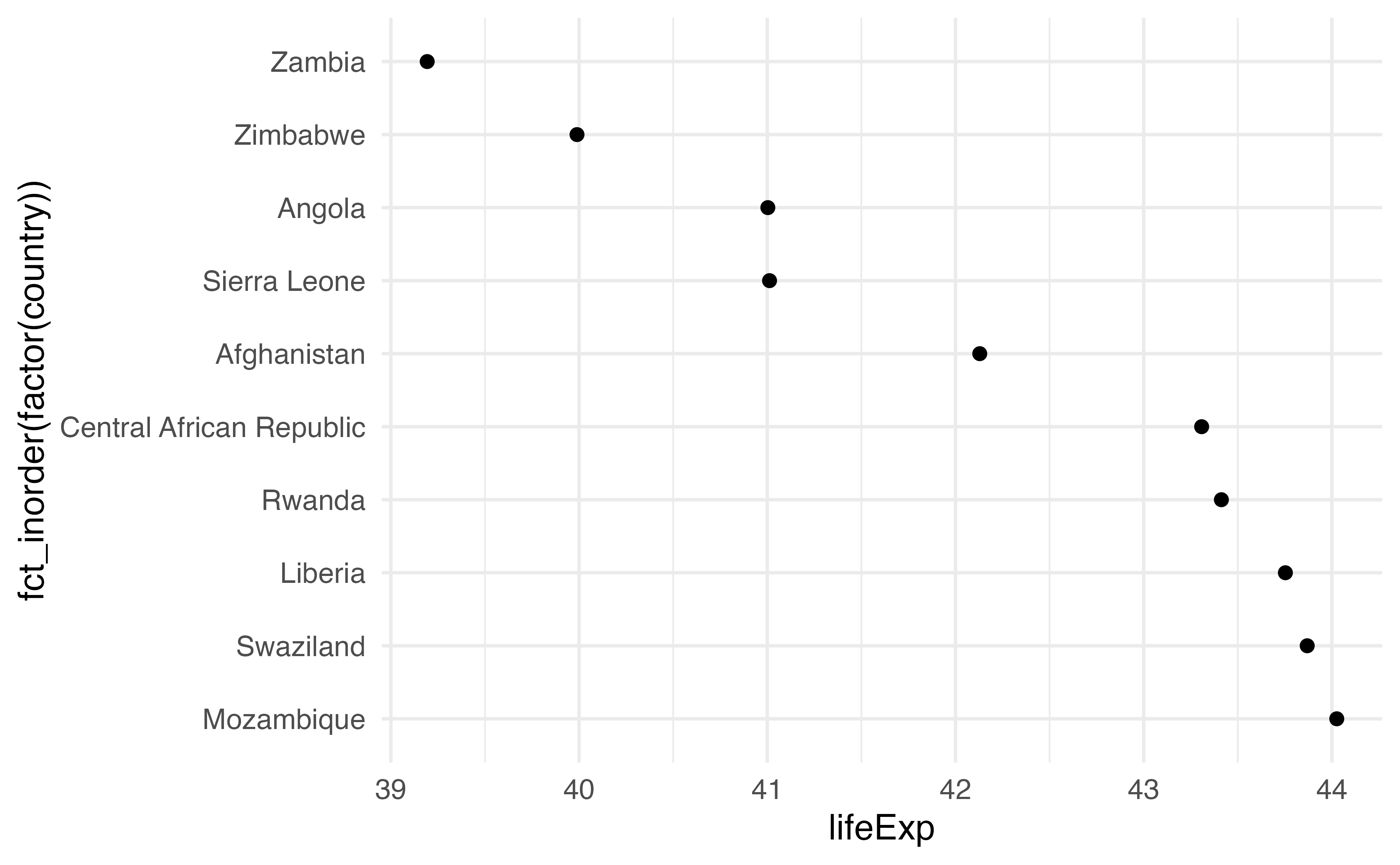
Make a scatter plot. Use variable for x. For y, we’ll use country, but to keep it in the order we arranged it by, we’ll turn it into a factor. Wrap the the factor() call with fct_inorder(). Check the help page if you want to know more about what this is doing.

Your turn 9

top_scatter_plot <- function(variable, .year) {
  gapminder |>
    filter(year == .year) |>
    arrange(desc({{ variable }})) |> 
    #  take the 10 lowest values
    tail(10) |> 
    ggplot(aes(
      x = {{ variable }}, 
      y = fct_inorder(factor(country))
    )) +
    geom_point() +
    theme_minimal()
}

Your turn 9

top_scatter_plot(lifeExp, 2002)

Your turn 9

top_scatter_plot(lifeExp, 2002) + 
  labs(x = "Life Expectancy", y = "Country")

Resources

R for Data Science, 2nd ed.: A comprehensive but friendly introduction to the Tidyverse. Free online.

Advanced R, 2nd ed.: Detailed guide to how R works and how to make your code better. Free online.